Understanding Dynamic Range

Devices

Portable balancer & Vibration analyzer Balanset-1A

€1,975.00 + VAT (if applicable)

Parts

Vibration sensor

€90.00 + VAT (if applicable)

Parts

Optical Sensor (Laser Tachometer)

€124.00 + VAT (if applicable)

Devices

Balanset-4

€6,803.00 + VAT (if applicable)

Parts

Magnetic Stand Insize-60-kgf

€46.00 + VAT (if applicable)

Parts

Reflective tape

€10.00 + VAT (if applicable)

Devices

Dynamic balancer “Balanset-1A” OEM

€1,735.00 + VAT (if applicable)

Dynamic range is the ratio between the largest and smallest signals a measurement system can handle accurately, usually expressed in decibels (dB). For a vibration measurement system it defines the span from the noise floor — the smallest signal that can be told apart from background noise — up to the saturation point, the largest signal before the system clips or distorts. A wide dynamic range lets one instrument setup capture both the faint tremor of an early bearing defect and the heavy shaking of severe unbalance at the same time.

This matters because real machinery vibration spans enormous amplitude ranges — from micro-g bearing-impact energy to multi-g unbalance forces — often in the same record. Adequate dynamic range is what guarantees that no diagnostic information either vanishes into the noise or saturates the front end, and it ranks alongside frequency range and sensitivity as a defining specification of any analyser.

1. How Dynamic Range Is Expressed

The decibel form is convenient because it compresses huge ratios into manageable numbers:

Dynamic range (dB) = 20 × log₁₀(maximum signal / minimum signal)

For example, a system that handles a maximum of 10 V over a minimum resolvable 1 mV has a dynamic range of 20 × log(10 / 0.001) = 80 dB. The same quantity can be stated as a plain ratio, which makes the scale intuitive:

• 80 dB ≈ 10,000 : 1
• 100 dB ≈ 100,000 : 1
• 120 dB ≈ 1,000,000 : 1

Every 20 dB therefore represents a tenfold widening of the measurable span — a useful rule of thumb when comparing instruments.

2. What Sets the Upper and Lower Limits

Upper limit: saturation

The top of the range is wherever the signal first clips:

• Sensor saturation: the maximum vibration the sensor itself can output cleanly.
• A/D converter saturation: the maximum voltage the digitiser accepts (±5 V or ±10 V are typical).
• Amplifier saturation: the signal-conditioning stages can clip before the converter does.

The effect of any of these is the same — the waveform tops out flat, and the spectrum sprouts false harmonics that were never in the machine.

Lower limit: the noise floor

The bottom of the range is set by the system’s own noise:

• Sensor noise: inherent electrical noise in the sensor electronics.
• Cable noise: interference picked up along the cable.
• Instrument noise: electronic noise inside the analyser.
• Quantisation noise: the irreducible rounding error of the A/D converter’s resolution.

Any genuine signal weaker than this floor is simply indistinguishable from noise.

3. Typical Dynamic Ranges

Both the sensor and the acquisition hardware constrain the system, and the achieved range is governed by whichever is narrower. As a guide:

Device	Typical dynamic range
IEPE accelerometers	80–100 dB
Charge-mode accelerometers	100–120 dB
Velocity transducers	60–80 dB
Proximity probes	60–80 dB
16-bit A/D	≈96 dB theoretical, 80–90 dB practical
24-bit A/D	≈144 dB theoretical, 110–120 dB practical
Modern analysers (system)	90–110 dB

The gap between the theoretical and practical figures for an A/D converter reflects real-world noise that erodes the last few bits, which is why a 24-bit converter delivers nothing like its 144 dB on paper.

4. Why It Matters in Vibration Analysis

The recurring challenge is measuring small and large signals at once. A spectrum may carry a towering 1× peak from unbalance and, beside it, the small peaks of an incipient bearing fault; the ratio between them can exceed 1000 : 1 (60 dB). With enough dynamic range both stay visible — with too little, the small peaks drown in noise or the large peak clips. The demand is even sharper in envelope analysis, which must pull low-energy bearing impacts out from under high-energy low-frequency vibration; band-pass filtering helps, but wide dynamic range remains essential for genuinely early detection. More generally, good spectral analysis wants to show dominant peaks and tiny diagnostic peaks together, which is exactly what an adequate range — viewed on a logarithmic scale — makes possible.

5. Optimising and Protecting Dynamic Range

You cannot change a system’s intrinsic range, but you can make the most of it. The three main levers are gain, sensor choice and filtering:

• Gain settings: set the input gain so the signal peaks fill the A/D range. Too little gain wastes resolution and leaves you near the noise limit; too much causes clipping. The practical target is to have peaks reach roughly 70–80% of full scale.
• Sensor selection: match sensor sensitivity to the expected vibration — high sensitivity for low-level machines, low sensitivity for heavy vibration — accepting a compromise when the range to be measured is very wide.
• Filtering: a high-pass filter that removes a dominant low-frequency component lets you raise the gain on what remains, effectively extending the usable dynamic range for high-frequency analysis — the very strategy envelope analysis relies on.

Two failure modes to recognise

Two practical problems sit at opposite ends of the range. Saturation (clipping) shows up as a flat-topped waveform and false harmonics in the spectrum; it is cured by reducing gain, fitting a lower-sensitivity sensor, or filtering out the large component, and most instruments offer a clipping indicator to warn you in advance. Noise limitation appears as an inability to track small changes and a generally noisy spectrum; it is eased by increasing gain, fitting a higher-sensitivity sensor, or improving cable routing and grounding.

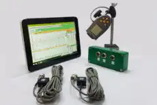
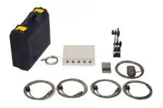
6. Display, Scaling and Field Practice

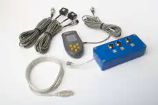
How the data is displayed determines how much of the captured range you can actually see. A linear amplitude scale offers only about 40–50 dB of useful display window, so small peaks disappear whenever a large peak is present — fine when the dynamic range in play is modest. A logarithmic (dB) scale, by contrast, can present the full dynamic range on a single plot, keeping both small and large peaks legible; it is the standard for detailed diagnostics and effectively indispensable for serious analysis. In the field, the same principles apply to a portable two-channel instrument such as the Balanset-1A: choosing a sensible gain, watching for clipping, and reading the spectrum on a log scale ensure that a single measurement captures both the dominant 1× amplitude and phase used for balancing and the faint high-frequency clues used for bearing screening.

In short, dynamic range is a fundamental specification of measurement capability. Understanding it, optimising it through correct gain and sensor choices, and respecting its limits is what allows an analyst to capture every layer of diagnostic information — from the subtlest early fault signature to the loudest mechanical vibration — in one reliable, comprehensive measurement.

---

← Back to Main Index