Understanding Bearing Fault Frequencies

Complete guide to BPFO, BPFI, BSF & FTF — the mathematically predictable vibration signatures that enable early bearing defect detection months before catastrophic failure.
Bearing Fault Frequency Calculator
Enter bearing parameters to calculate all four characteristic frequencies
Calculated Frequencies
Results update after clicking Calculate
to see fault frequencies
Quick Reference — The Four Fault Frequencies
Summary cards and comparison tables for rapid identification during vibration analysis
| Parameter | BPFO (Outer Race) | BPFI (Inner Race) | BSF (Ball/Roller) | FTF (Cage) |
|---|---|---|---|---|
| Frequency Range | 3–5× RPM | 5–7× RPM | 1.5–3× RPM | 0.35–0.45× RPM |
| Failure Probability | ~40% of failures | ~30% of failures | ~10% of failures | ~20% of failures |
| Sideband Pattern | 1× sidebands (if loose) | ±1×, ±2× sidebands (always) | Sidebands at FTF spacing | Random, often erratic |
| Detection Difficulty | Easy | Moderate | Hard | Hard |
| Best Detection Method | Standard FFT | Envelope analysis | Envelope analysis | Time waveform + envelope |
| Typical Cause | Fatigue, contamination, overload | Fatigue, shaft misalignment | Manufacturing defect, overload | Poor lubrication, wear |
| Load Zone Effect | Fixed (defect in load zone = higher amp) | Modulated (enters/exits zone) | Double impact per revolution | May fluctuate randomly |
| Stage | Spectrum Indicators | Other Indicators | Typical Time to Failure | Recommended Action |
|---|---|---|---|---|
| Stage 1 — Early | Faint peaks near noise floor; visible only in envelope spectrum | No audible noise; temperature normal; ultrasound may detect | 6–24 months | Monitor monthly; plan procurement |
| Stage 2 — Developing | Clear fault frequency peaks + 2–3 harmonics in standard FFT | Possible slight temperature rise; intermittent noise at high load | 1–6 months | Monitor bi-weekly; schedule replacement |
| Stage 3 — Advanced | High-amplitude peaks, many harmonics, sideband families, rising noise floor | Audible noise; temperature rise; visible vibration; grease discoloration | 1–4 weeks | Replace at earliest opportunity |
| Stage 4 — Critical | Chaotic spectrum; broadband energy; sub-harmonic peaks; 1× RPM change | Loud noise; high temperature; smoke possible; metal debris in grease | Days to hours | Immediate shutdown and replacement |
| Bearing | Type | N (Balls) | BPFO (Hz) | BPFI (Hz) | BSF (Hz) | FTF (Hz) |
|---|
Definition: What Are Bearing Fault Frequencies?
Bearing fault frequencies (also called bearing defect frequencies or characteristic frequencies) are specific vibration frequencies generated when rolling elements—balls or rollers—in a bearing pass over defects such as cracks, spalls, pits, or surface fatigue on the bearing races or the rolling elements themselves. These frequencies are mathematically predictable based on the bearing's internal geometry and the shaft's rotational speed, making them invaluable diagnostic indicators for early detection of bearing defects.
Understanding and identifying these frequencies through vibration analysis allows maintenance personnel to detect bearing problems months—sometimes years—before they would become apparent through temperature rise, audible noise, or catastrophic failure. This enables planned maintenance and prevents costly unplanned downtime, secondary damage to shafts and housings, and potential safety incidents.
Unlike many vibration sources that produce unpredictable frequencies, bearing fault frequencies can be calculated precisely from bearing geometry. This means an analyst can know exactly which frequencies to look for in a spectrum, eliminating guesswork and enabling automated monitoring systems that continuously watch for these specific signatures.
The Four Fundamental Fault Frequencies — In Depth
Every rolling element bearing has four characteristic fault frequencies. Each corresponds to a different type of defect on a specific bearing component. Understanding the physical mechanism behind each frequency is essential for accurate diagnosis.
1. BPFO — Ball Pass Frequency, Outer Race
The BPFO represents the rate at which rolling elements pass over a fixed point on the outer race. When a defect exists on the outer raceway surface, each rolling element strikes the defect as it passes, generating a repetitive impact at a predictable frequency.
Physical Mechanism
In most bearing installations, the outer race is stationary (pressed into the housing). This means that a defect on the outer race stays in a fixed position relative to the load zone—the arc where the shaft load is transferred through the rolling elements. Because the defect's position doesn't change relative to the load, the impact force at each rolling element passage remains relatively constant. This produces a clean, strong vibration signal that is generally the easiest bearing defect to detect.
Diagnostic Characteristics
- Typical range: 3–5× shaft speed for most standard bearings
- Amplitude consistency: Relatively uniform amplitude because the defect is always in the same position relative to the load zone
- Sideband behavior: Minimal sidebands in typical installations; 1× sidebands may appear if the outer race can rotate slightly in its housing (loose fit)
- Harmonic development: As the defect grows, 2×, 3×, 4× BPFO harmonics appear progressively
- Detection ease: Easiest of the four fault types to detect due to consistent signal amplitude
If a BPFO peak is present but weak, the defect may be located outside the primary load zone. Changing the measurement direction (e.g., from vertical to horizontal) or changing the load on the bearing can move the load zone relative to the defect, potentially making it more visible in the spectrum.
2. BPFI — Ball Pass Frequency, Inner Race
The BPFI represents the rate at which rolling elements pass over a fixed point on the inner race. Since the inner race rotates with the shaft, a defect on the inner race moves in and out of the load zone with each revolution—a critical difference from outer race defects.
Physical Mechanism
The inner race is press-fitted onto the shaft and rotates with it. A spall or pit on the inner race surface is struck by each rolling element as it passes, but unlike BPFO, the impact energy varies as the defect travels through the loaded and unloaded zones of the bearing. When the defect is in the load zone (bottom of a horizontal shaft bearing), the rolling elements are pressed firmly against both races, and the impact is strong. When the defect rotates to the unloaded zone (top), the rolling elements barely contact the inner race, and the impact may be very weak or absent.
This amplitude modulation at 1× shaft speed is the defining signature of inner race defects and produces characteristic sidebands in the frequency spectrum.
Diagnostic Characteristics
- Typical range: 5–7× shaft speed (always higher than BPFO for the same bearing)
- Amplitude modulation: Signal amplitude modulated at shaft speed (1×) as defect enters/exits load zone
- Sideband behavior: Almost always shows ±1×, ±2× sidebands around BPFI — this is the key diagnostic indicator
- Detection difficulty: Harder than BPFO because of varying amplitude; envelope analysis is often required for early detection
- Common causes: Shaft misalignment creating uneven stress, improper interference fit, shaft deflection fatigue
The presence of 1× sidebands around BPFI is often more diagnostically significant than the BPFI peak itself. In early-stage inner race defects, the sidebands may be more prominent than the fundamental BPFI frequency. Always check for sideband families when investigating inner race conditions.
3. BSF — Ball Spin Frequency
The BSF represents the rotational speed of a rolling element (ball or roller) spinning on its own axis. When a rolling element has a surface defect—a pit, spall, or flat spot—it impacts both the inner and outer raceways as it rotates, creating a distinctive but complex vibration pattern.
Physical Mechanism
Each rolling element in a bearing spins on its own axis as it orbits around the bearing center. The spin rate depends on the ratio of pitch diameter to ball diameter and the shaft speed. A defect on a rolling element strikes the outer race once per ball revolution when it faces outward, and the inner race once per ball revolution when it faces inward. This produces impacts at 2× BSF (two impacts per revolution of the defective element). Additionally, because the defective rolling element is carried around the bearing by the cage, its signal is modulated at the cage frequency (FTF).
Diagnostic Characteristics
- Typical range: 1.5–3× shaft speed
- Signature frequency: Often appears as 2× BSF rather than 1× BSF (double impact per revolution)
- Sideband behavior: Sidebands at FTF (cage frequency) spacing around BSF peaks
- Detection difficulty: Most difficult bearing defect to detect; rolling elements can develop flats that "self-heal" by re-polishing, causing intermittent symptoms
- Occurrence rate: Less common than race defects; often a manufacturing or contamination issue
4. FTF — Fundamental Train Frequency
The FTF represents the rotational speed of the bearing cage (also called the retainer or separator). The cage holds the rolling elements in proper spacing around the bearing and rotates at a fraction of shaft speed.
Physical Mechanism
The cage rotates at a speed between 0 and shaft speed—typically around 0.35–0.45× shaft speed. Cage failures produce sub-synchronous vibration that can be erratic and difficult to distinguish from other low-frequency sources. Cage problems usually stem from inadequate lubrication, which causes the cage to drag against the rolling elements or races, creating wear, deformation, or cracking.
Diagnostic Characteristics
- Typical range: 0.35–0.45× shaft speed (sub-synchronous)
- Signal character: Often erratic and non-repetitive, making it harder to detect with standard FFT averaging
- Modulation: May modulate other bearing frequencies — look for FTF sidebands around BPFO or BPFI
- Detection: Best detected using time waveform analysis combined with envelope analysis; may also appear in shaft orbit patterns
- Risk level: Cage failures can be catastrophic because cage fragments can jam the bearing, causing sudden seizure
Unlike race defects that progress gradually, cage failures can escalate rapidly from minor to catastrophic. If FTF activity is detected, especially with erratic or broadband characteristics, increased monitoring frequency is strongly recommended. Cage fragment can cause sudden bearing seizure, potentially leading to shaft damage, equipment wreck, and safety hazards.
Formula Variables and Calculations Explained
The fault frequency formulas use the bearing's internal geometric parameters. These dimensions define the relationship between shaft rotation and the movement of each bearing component:
| Variable | Name | Description | Units |
|---|---|---|---|
| N | Number of rolling elements | Total count of balls or rollers in the bearing | — |
| n | Shaft rotational frequency | Rotational speed of the inner race / shaft | Hz or RPM |
| Bd | Ball / roller diameter | Diameter of one rolling element | mm or inches |
| Pd | Pitch diameter | Diameter of the circle passing through centers of all rolling elements | mm or inches |
| β | Contact angle | Angle between line connecting ball-race contact points and bearing radial plane. 0° for deep groove, 15–40° for angular contact and tapered roller. | degrees |
Most vibration analysis software includes bearing databases with pre-calculated parameters for tens of thousands of bearing models from all major manufacturers (SKF, FAG, NSK, NTN, Timken, etc.). Alternatively, manufacturer catalogs and online tools provide Bd, Pd, N, and β for any bearing designation. For very old or uncommon bearings, the parameters can be estimated from measured outer diameter, inner bore, and bearing width.
Simplified Estimation Rules
When exact bearing geometry is unavailable, these approximations work reasonably well for most standard deep groove ball bearings with contact angle ≈ 0°:
- BPFO ≈ 0.4 × N × shaft speed — reliable within ±5% for most bearings
- BPFI ≈ 0.6 × N × shaft speed — reliable within ±5%
- FTF ≈ 0.4 × shaft speed — reliable within ±10%
- BSF varies too widely to estimate without geometry
These approximations are useful for field diagnostics when a bearing database is not available, but precise calculations should always be used for formal analysis reports and trending programs.
How Fault Frequencies Appear in Vibration Spectra
Understanding how bearing defects manifest in the frequency domain is crucial for accurate diagnosis. The spectral pattern changes significantly as a defect progresses through its life cycle.
Basic Spectral Appearance
When a bearing develops a localized defect (spall, crack, or pit), each passage of a rolling element over the defect generates a short-duration impact. This impact excites the bearing's natural resonance frequencies (typically 1–30 kHz range), creating a modulated high-frequency signal. In the frequency spectrum, this appears as:
- Primary peak: A distinct peak at the calculated fault frequency
- Harmonics: Additional peaks at 2×, 3×, 4× the fault frequency, increasing in number as the defect grows
- Sidebands: Satellite peaks flanking the fault frequency, spaced at modulating frequency intervals
- Amplitude growth: Progressive increase in fault frequency amplitude as defect area increases
Sideband Patterns — Key Diagnostic Signatures
Sidebands are secondary peaks that appear around a primary fault frequency, spaced at intervals determined by the modulating mechanism. They provide crucial information for confirming which bearing component is defective:
- Inner race defects: BPFI peak with sidebands at ±1×, ±2×, ±3× shaft speed. This is caused by the defect rotating through the load zone once per shaft revolution, modulating the impact energy.
- Outer race defects: BPFO peak usually without sidebands in normally fitted bearings. If sidebands at 1× shaft speed appear around BPFO, it may indicate the outer race is able to rotate slightly in its housing (loose fit condition).
- Rolling element defects: BSF peaks (often 2× BSF) with sidebands spaced at FTF (cage frequency). The cage carries the defective element around the bearing, causing the defect's position relative to the load zone to change at the cage rotation rate.
- Cage defects: FTF peak, often with harmonics, may show erratic amplitude variations. Cage frequency sidebands around BPFO or BPFI can indicate cage-related problems affecting rolling element spacing.
Defect Progression Stages
Bearing defects progress through recognizable stages, each with characteristic spectral patterns:
Detection Techniques — From Simple to Advanced
Standard FFT Analysis
The Fast Fourier Transform is the fundamental tool for vibration spectrum analysis. For bearing diagnostics, the procedure involves calculating the FFT of the raw vibration signal and examining it for peaks at the calculated bearing fault frequencies.
Standard FFT analysis is effective for moderate to advanced defects (Stages 2–4) where fault frequency energy is strong enough to stand out above the noise floor and other vibration sources. However, it has significant limitations for early detection because bearing fault signals are typically low-energy, high-frequency impacts that can be masked by stronger low-frequency vibration from imbalance, misalignment, and other sources.
Envelope Analysis (Demodulation) — The Gold Standard
Envelope analysis (also called High Frequency Demodulation or HFD) is the most effective technique for early bearing defect detection. It works by exploiting the physical nature of bearing impacts:
- Step 1 — Band-pass filter: The raw vibration signal is filtered to isolate the high-frequency range (typically 500 Hz – 20 kHz) where bearing impacts excite structural resonances. This removes dominant low-frequency vibration from imbalance, misalignment, etc.
- Step 2 — Rectification: The filtered signal is rectified (absolute value) or passed through a Hilbert transform to extract the amplitude envelope.
- Step 3 — Envelope FFT: The FFT of the envelope signal reveals the repetition rate of the impacts — which corresponds directly to bearing fault frequencies.
Envelope analysis can detect bearing faults 6–12 months earlier than standard FFT methods, making it the preferred technique for predictive maintenance programs. Most modern vibration analyzers include this capability as a standard feature.
Time-Domain Techniques
- Shock Pulse Method (SPM): Measures the intensity of mechanical shock waves generated by metal-to-metal impact in rolling bearings. Uses a resonant transducer (typically 32 kHz) to detect the short-duration, high-energy impacts from surface defects. Reports dBsv (decibels shock value) with normalised dBn and dBc values comparing to new and damaged bearing thresholds.
- Crest Factor: The ratio of peak vibration amplitude to RMS amplitude. A healthy bearing has a crest factor around 3; as impacting begins from surface defects, peak values increase while RMS stays relatively constant, pushing crest factor to 5–7 or higher. Note: in late-stage failure, both peak and RMS increase, and crest factor may drop back toward normal — a potential trap for unwary analysts.
- Kurtosis: A statistical measure of the "peakedness" of the vibration signal distribution. A normal (Gaussian) signal has kurtosis = 3. Early bearing defects create sharp impacts that increase kurtosis to 4–8 or higher, making it a sensitive early indicator. Like crest factor, kurtosis may decrease in late-stage failure as the signal becomes broadband.
Advanced Techniques
- Spectral Kurtosis: Maps kurtosis values across frequency bands to identify the optimal demodulation band for envelope analysis, replacing guesswork in filter selection.
- Minimum Entropy Deconvolution (MED): Signal processing technique that enhances impulsiveness in vibration data, improving detection of periodic impacts from bearing faults in noisy signals.
- Cyclostationary Analysis: Exploits the second-order cyclostationary properties of bearing fault signals (periodic modulation of random noise), providing superior detection in very early defect stages.
- Wavelet Analysis: Time-frequency decomposition that can isolate transient bearing impacts in both time and frequency simultaneously, useful when conventional methods are inconclusive.
Practical Application — Step-by-Step Diagnostic Procedure
Identify Bearing
Determine the bearing model number and exact location. Check equipment drawings, bearing housing markings, or maintenance records. The model number is essential for calculating correct fault frequencies.
Calculate Fault Frequencies
Use the bearing geometry parameters (N, Bd, Pd, β) and current shaft speed to calculate BPFO, BPFI, BSF, and FTF. Use the calculator above, bearing database software, or the formulas directly. Note: shaft speed may vary — measure actual RPM if possible.
Collect Vibration Data
Mount an accelerometer on the bearing housing as close to the load zone as possible. Measure acceleration in all three axes. Use a sampling rate at least 10× the highest frequency of interest (for envelope analysis, sample at 40–100 kHz). Ensure the machine is running at normal operating load and speed.
Analyze Spectrum
Examine both the standard FFT spectrum and the envelope spectrum for peaks at calculated fault frequencies. Look for BPFO, BPFI, BSF, and FTF and their harmonics. Use cursor read-out to verify frequencies match within ±2% of calculated values (allow for slight speed variation).
Confirm Diagnosis with Sidebands
Check for sideband patterns consistent with the identified defect type. BPFI should show 1× sidebands; BSF should show FTF sidebands. The presence of correct sidebands confirms the diagnosis and distinguishes bearing frequencies from other coincidental peaks.
Assess Severity
Evaluate the defect stage based on amplitude, number of harmonics, sideband development, noise floor elevation, and comparison with baseline/historical data. Classify as Stage 1–4 using the severity guide above.
Plan Maintenance Action
Based on severity assessment and equipment criticality, schedule bearing replacement during the next available maintenance window. Stages 1–2 allow extended monitoring; Stage 3 requires near-term planning; Stage 4 demands immediate attention. Document findings for trending purposes.
Worked Example — Complete Diagnosis
Machine: 22 kW, 4-pole, 50 Hz induction motor driving a centrifugal pump. Operating speed: 1470 RPM (24.5 Hz). Drive-end bearing: SKF 6308 deep groove ball bearing.
Bearing Data: N = 8 balls, Bd = 15.875 mm, Pd = 58.5 mm, β = 0°. Bd/Pd ratio = 0.2714.
Calculated Frequencies:
- BPFO = (8 × 24.5 / 2) × (1 + 0.2714) = 98.0 × 1.2714 = 124.6 Hz
- BPFI = (8 × 24.5 / 2) × (1 − 0.2714) = 98.0 × 0.7286 = 71.4 Hz — Wait, this doesn't seem right. Let's recalculate properly:
Note: BPFI uses (1 − Bd/Pd) while BPFO uses (1 + Bd/Pd). BPFI should always be higher than BPFO. Looking at the standard formulas, in the canonical formulations where the outer race is fixed:
- BPFO = (N/2) × n × (1 − Bd/Pd × cos β) = 4 × 24.5 × (1 − 0.2714) = 98.0 × 0.7286 = 71.4 Hz
- BPFI = (N/2) × n × (1 + Bd/Pd × cos β) = 4 × 24.5 × (1 + 0.2714) = 98.0 × 1.2714 = 124.6 Hz
- BSF = (Pd/(2×Bd)) × n × [1 − (Bd/Pd)² × cos² β] = (58.5/31.75) × 24.5 × [1 − 0.0737] = 1.8425 × 24.5 × 0.9263 = 41.8 Hz
- FTF = (n/2) × (1 − Bd/Pd × cos β) = 12.25 × 0.7286 = 8.9 Hz
Measurement Results (Envelope Spectrum): A prominent peak at 124.3 Hz (matching BPFI within 0.2%) with harmonics at 248.7 Hz and 373.1 Hz. Sideband peaks at 99.8 Hz and 148.8 Hz (±24.5 Hz = ±1× shaft speed around BPFI).
Diagnosis: Inner race defect confirmed — BPFI fundamental with 1× sidebands is the classic signature. The presence of 2 harmonics but clear sideband structure indicates Stage 2–3 defect progression.
Recommended Action: Schedule bearing replacement within 2–4 weeks. Continue monitoring weekly until replacement. Inspect removed bearing for root cause (misalignment? improper fit? lubrication?). Verify alignment and fit during reinstallation.
Importance for Predictive Maintenance
Bearing fault frequencies form the cornerstone of effective predictive maintenance programs for rotating equipment. Their impact on maintenance strategy is profound:
- Early Warning — 6 to 24 Months Lead Time: Envelope analysis can detect bearing defects at the earliest stage of surface fatigue, providing months or even years of advance warning. This completely eliminates surprise failures and allows strategic procurement, staffing, and scheduling of maintenance activities.
- Specific Component Diagnosis: Unlike overall vibration level monitoring, which can only say "something is wrong," fault frequency analysis identifies exactly which bearing component is damaged — outer race, inner race, rolling element, or cage. This specificity enables precise repair scoping and parts ordering.
- Trend Monitoring and Remaining Life Prediction: By tracking fault frequency amplitudes over time, analysts can establish deterioration rates and predict when a bearing will reach end of life. This trending capability enables just-in-time replacement—not too early (wasting remaining bearing life) and not too late (risking failure).
- Root Cause Analysis: The pattern of bearing defects across a machine fleet reveals systemic issues. Frequent outer race defects may indicate contamination; inner race defects may indicate shaft misalignment patterns; rolling element defects may indicate a bad batch from a supplier.
- Secondary Damage Prevention: A failed bearing can destroy the shaft journal, damage the housing bore, wreck seal surfaces, contaminate lubricating systems, and even cause fire or explosion in hazardous environments. Early detection and planned replacement prevents all secondary damage.
- Documented Cost Savings: Studies consistently show that predictive maintenance based on vibration analysis returns 10:1 or higher cost-benefit ratios compared to reactive (run-to-failure) maintenance. For critical equipment, the savings are even higher when production losses from unplanned downtime are included.
Leading maintenance programs combine routine vibration data collection (monthly or quarterly for most equipment) with automated alarm systems that continuously monitor critical machines. Bearing fault frequencies should be configured as alarm parameters in online monitoring systems, with alert thresholds set based on historical baselines. This two-tier approach catches both gradual deterioration and sudden-onset defects.
Bearing fault frequencies are among the most powerful and well-proven diagnostic tools in vibration analysis. Their mathematical predictability, combined with modern envelope analysis and automated monitoring technology, enables reliable early detection of bearing defects. Mastering these concepts is essential for anyone involved in condition monitoring, reliability engineering, or predictive maintenance of rotating equipment.
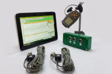
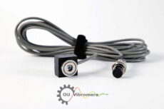
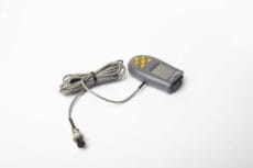
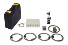
Professional Vibration Analysis Equipment
Detect bearing faults early with Vibromera's portable balancing and vibration analysis devices — professional capabilities at accessible prices.
Browse Equipment →