Understanding Natural Frequency


The inherent vibration frequency of every physical structure — and why its relationship with resonance is one of the most critical concepts in vibration analysis and rotating machinery engineering.
Natural Frequency Calculator
Calculate fn for simple systems + check resonance risk against operating speed
Results
Natural frequency and resonance risk assessment
to see the natural frequency
Key Concepts — At a Glance
The three fundamental properties that govern every vibrating system
| Structure / Component | Typical fn Range | Typical Operating RPM | Resonance Risk | Notes |
|---|---|---|---|---|
| Large concrete foundation | 15–40 Hz | 900–2400 | Low | Very stiff; typically well above operating speed |
| Steel baseplate / skid | 20–80 Hz | 1200–4800 | Medium | Can coincide with 2-pole or 4-pole motor speed |
| Piping system (span) | 5–50 Hz | 300–3000 | High | Long unsupported spans are very susceptible |
| Pump pedestal | 25–60 Hz | 1500–3600 | Medium | Vertical pumps are especially problematic |
| Fan housing / shroud | 15–120 Hz | 900–7200 | Medium | Sheet metal panels can have many modes |
| Electric motor frame | 40–200 Hz | 2400–12000 | Low | Typically designed above 1× operating speed |
| Shaft (1st critical) | 20–500 Hz | 1200–30000 | High | Must be known; crossing critical = severe vibration |
| Bearing housing | 100–1000 Hz | — | Low | Excited by bearing fault impacts, not by 1× speed |
| Gearbox casing | 200–2000 Hz | — | Low | Excited by gear meshing frequencies |
| Spring isolators (installed) | 2–8 Hz | 120–480 | Medium | Must be well below operating speed to isolate |
| Rubber mounts | 5–25 Hz | 300–1500 | Medium | Stiffness varies with temperature and age |
| Frequency Ratio (fop / fn) | Zone | Amplification Factor | Practical Meaning | Recommendation |
|---|---|---|---|---|
| 0 – 0.7 | Safe Below | 1.0 – 2.0× | Vibration force transmitted almost 1:1; structure moves in-phase with forcing | Acceptable; normal operating zone for rigidly mounted equipment |
| 0.7 – 0.85 | Approach Zone | 2 – 5× | Amplitude begins to amplify significantly; early resonance effects | Avoid steady-state operation; acceptable for brief run-up/coast-down transit |
| 0.85 – 1.15 | Resonance Band | 5 – 50× | Severe amplification; amplitude limited only by damping; structural damage possible | Never operate here; transit through quickly if unavoidable |
| 1.15 – 1.4 | Exit Zone | 2 – 5× | Amplitude decreasing but still elevated; phase shifting rapidly | Avoid steady-state; brief transit acceptable |
| 1.4 – 2.5 | Safe Above | 0.3 – 1.0× | Vibration is attenuated; structure's inertia resists movement; phase inversion | Good isolation zone for flexibly mounted equipment |
| > 2.5 | Isolation Zone | < 0.3× | Excellent vibration isolation; very little force transmitted | Ideal for spring/rubber-mounted machines |
| Method | Equipment Needed | Machine State | Accuracy | Best For | Limitations |
|---|---|---|---|---|---|
| Impact Test (Bump Test) | Modal hammer + accelerometer + FFT analyzer | Stopped | High | Structures, baseplates, piping, bearing housings | Machine must be stopped; can miss speed-dependent effects |
| Run-Up / Coast-Down | Vibration sensor + tachometer + order tracking | Running (variable speed) | High | Shaft critical speeds, foundation resonances | Requires variable speed; 1× unbalance force excites primarily shaft criticals |
| Operating Deflection Shape (ODS) | Multi-channel analyzer + many sensors | Running (normal) | Medium | Visualizing how structure moves at specific frequency | Shows deflection shape, not true mode shape (multiple modes contribute) |
| Experimental Modal Analysis (EMA) | Modal hammer or shaker + roving sensors + modal software | Stopped | Very High | Complete modal model (frequencies, shapes, damping) | Time-consuming; requires expertise; complex data processing |
| Finite Element Analysis (FEA) | Computer + FEA software + model | N/A (simulation) | Depends on model | Design phase; what-if analysis; complex geometries | Accuracy depends on model quality; boundary conditions critical |
| Waterfall / Cascade Plot | Vibration analyzer with order tracking | Running (variable speed) | High | Identifying multiple resonances during speed changes | Requires speed change; only finds resonances excited by operating forces |
Definition: What is Natural Frequency?
Natural frequency is the frequency at which a mechanical system oscillates freely after being displaced from equilibrium. It is determined by the system's mass and stiffness: fn = (1/2π) × √(k/m), where k is stiffness (N/m) and m is mass (kg). When an external force frequency matches a natural frequency, resonance occurs — vibration amplitude can increase 10–50× and cause catastrophic failure. In rotating machinery, the critical speed (RPM) = fn × 60. A quick field estimate uses static deflection: fn ≈ 15.76 / √δmm.
A natural frequency is the specific frequency at which a physical object or system will oscillate when disturbed from its equilibrium position and then allowed to vibrate freely, without any ongoing external driving force. It is an inherent, fundamental property of the object, determined entirely by its physical characteristics — principally its mass (inertia) and its stiffness (elasticity). Every physical object, from a guitar string to a bridge span to a machine's support pedestal, possesses one or more natural frequencies.
Natural frequencies are sometimes called eigenfrequencies (from the German word "eigen" meaning "own" or "characteristic"), and the corresponding vibration patterns are called mode shapes or eigenmodes. A complex structure like a machine base may have hundreds of natural frequencies, each associated with a unique deformation pattern — bending, twisting, breathing, rocking, and so on.
In rotating machinery, vibration problems are frequently caused not by excessive excitation forces (such as unbalance), but by the unlucky coincidence of an excitation frequency matching a structural natural frequency. A perfectly acceptable amount of unbalance can produce destructive vibration if the machine operates at or near a structural resonance. Identifying natural frequencies is therefore one of the most important diagnostic steps when investigating unexplained high vibration.
The Relationship Between Mass, Stiffness, and Natural Frequency
The fundamental relationship between mass, stiffness, and natural frequency is one of the most important concepts in vibration engineering. It is both intuitive and mathematically precise.
Intuitive Understanding
- Stiffness (k): A stiffer object has a higher natural frequency. Think of a guitar string: tightening the string (increasing tension/stiffness) raises the pitch (frequency). A thick steel beam vibrates at a much higher frequency than a thin aluminum strip of the same length.
- Mass (m): A more massive object has a lower natural frequency. Think of a ruler extending off the edge of a desk: a longer, heavier ruler oscillates more slowly (lower frequency) than a shorter, lighter one. Adding weight to a structure always lowers its natural frequencies.
The Fundamental Formula
For a simple single-degree-of-freedom (SDOF) system — a mass connected to a spring — the undamped natural frequency is:
This formula has profound practical implications:
- To increase fn by 2×, you must increase stiffness by 4× (because of the square root) — or reduce mass by 4×
- To decrease fn by 2×, you must reduce stiffness by 4× — or increase mass by 4×
- Changes to stiffness and mass have diminishing returns: each doubling of fn requires a 4× change in the parameter
The Static Deflection Shortcut
One of the most useful practical formulas in vibration engineering relates natural frequency directly to static deflection under gravity:
This is remarkably useful because static deflection is often easy to measure or estimate: simply measure how much a structure deflects under the weight of the machine. A machine that sags 1 mm on its supports has a vertical natural frequency of about 15.8 Hz (948 RPM). A machine that sags 0.25 mm has fn ≈ 31.5 Hz (1890 RPM).
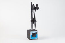
Need a quick natural frequency estimate without instruments? Place a dial indicator under the machine's bearing housing and observe the static deflection when the machine weight is applied (e.g., during installation). The formula fn ≈ 15.76/√δmm gives a remarkably good first approximation of the fundamental vertical natural frequency.
Multiple Degrees of Freedom
Real structures are not simple SDOF systems — they have many masses connected through distributed stiffness, resulting in many natural frequencies. A simple rigid body on elastic supports has six natural frequencies corresponding to six degrees of freedom: three translational (vertical, lateral, axial) and three rotational (roll, pitch, yaw). A flexible structure has infinitely many modes, though only the lowest several are usually of practical concern.
The key principle is: the number of natural frequencies equals the number of degrees of freedom in the model. A simple beam modeled with 10 lumped masses has 10 natural frequencies; a finite element model with 10,000 nodes has 30,000 (3 DOF per node) natural frequencies, though only a few dozen may be in the frequency range of interest.
The Effect of Damping
Real systems always have some damping — friction, material hysteresis, radiation into surrounding structure, fluid drag, etc. Damping has two effects:
- Slightly lowers the actual resonant frequency: The damped natural frequency is fd = fn × √(1 − ζ²), where ζ is the damping ratio. For typical mechanical structures (ζ = 0.01–0.05), this effect is negligible — less than 0.1% reduction.
- Limits the amplitude at resonance: Without damping, resonance amplitude would theoretically be infinite. The amplification factor Q (quality factor) at resonance is approximately Q = 1/(2ζ). For a lightly damped structure with ζ = 0.02, Q = 25 — meaning the vibration amplitude at resonance is 25× what it would be away from resonance. This is why even small amounts of unbalance can produce enormous vibration at critical speeds.
Natural Frequency and Resonance: The Critical Connection
The concept of natural frequency is critically important in engineering specifically because of its direct connection to the phenomenon of resonance.
What is Resonance?
Resonance occurs when a periodic external force is applied to a system at a frequency that is equal to or very close to one of its natural frequencies. When this happens, the system absorbs energy from the external force with maximum efficiency, causing the vibration amplitude to grow dramatically. Each cycle of the forcing function adds energy to the system in exact synchronization with the system's natural oscillation, building amplitude cycle after cycle until either damping limits further growth or the structure fails.
The Amplification Factor
The magnification of vibration at resonance depends critically on the system's damping. The dynamic magnification factor (DMF) describes how much larger the dynamic response is compared to the static deflection that the same force would produce:
| Damping Ratio (ζ) | Typical System | Q Factor (≈ 1/2ζ) | Amplification at Resonance |
|---|---|---|---|
| 0.005 | Welded steel structure, undamped | 100 | 100× static deflection |
| 0.01 | Steel frame, bolted connections | 50 | 50× static deflection |
| 0.02 | Typical machinery structure | 25 | 25× static deflection |
| 0.05 | Concrete foundation, bolted joints | 10 | 10× static deflection |
| 0.10 | Rubber-mounted, well-damped | 5 | 5× static deflection |
| 0.20 | Highly damped (viscous damper) | 2.5 | 2.5× static deflection |
Why Resonance Is Dangerous
Resonance is particularly treacherous because the vibration amplitude can be 10–100× larger than expected based on the forcing magnitude alone. A rotor with 50 µm of unbalance eccentricity that produces 1 mm/s vibration at non-resonant speed could produce 25–50 mm/s at resonance — enough to destroy bearings, fatigue bolts, crack welds, and cause cascading equipment failure.
The collapse of the Tacoma Narrows Bridge remains one of the most dramatic demonstrations of resonance in engineering history. Wind forces at a frequency near the bridge's torsional natural frequency caused the bridge deck to oscillate with increasing amplitude until structural failure occurred. The event led to fundamental changes in bridge engineering and is studied in every structural dynamics course worldwide. Modern engineers routinely perform modal analysis to ensure structures are designed away from foreseeable excitation frequencies.
Critical Speeds of Rotating Machinery
In rotating machinery, the most important manifestation of natural frequency is the critical speed — the rotational speed at which the shaft's rotation frequency (1× RPM) coincides with a natural frequency of the rotor-bearing-support system. When a machine operates at a critical speed, the 1× unbalance force excites the natural frequency, producing severe resonant vibration.
Types of Critical Speeds
- Rigid body criticals: Occur when the shaft speed matches a natural frequency of the rotor on its bearing supports, with the shaft itself remaining essentially straight. These are typically the first and second criticals (bounce and rock modes) and occur at lower speeds. Rigid body criticals can be modified by changing bearing stiffness or support structure mass.
- Flexible rotor criticals (bending criticals): Occur when the shaft speed matches a natural frequency associated with shaft bending deformation. The first bending critical typically involves the shaft bowing into a half-sine shape. These are more dangerous because they involve large deflections at the shaft midspan and cannot be controlled by bearing changes alone — the shaft geometry itself must be modified.
Separation Margin
Industry standards (e.g., API 610, API 617) require a minimum separation margin between operating speed and critical speeds:
- API typical requirement: Operating speed must be at least 15–20% away from any lateral critical speed (undamped)
- General good practice: A 20% margin is considered minimum; 30% is preferred for critical equipment
- VFD-driven equipment: Variable frequency drives change operating speed, potentially sweeping through criticals. The entire operating range must be checked, and criticals within the range must be identified and excluded or rapid transit programmed.
When field balancing a machine that operates near (but safely above) a critical speed, the phase relationship between unbalance and vibration response will differ from what is expected for a "below-resonance" machine. The vibration signal may be 90–180° ahead of the heavy spot rather than in-phase. Good balancing equipment handles this automatically through trial-weight response measurement, but the analyst should be aware that near-critical operation complicates simple vector analysis.
How Are Natural Frequencies Identified?
Identifying the natural frequencies of a machine or structure is a fundamental diagnostic skill. Several methods are available, ranging from simple to sophisticated:
1. Impact Testing (Bump Test)
The most common and practical experimental method for identifying structural natural frequencies. The procedure involves striking the machine or structure (while it is not running) with an instrumented impact hammer and measuring the resulting vibration with an accelerometer. The hammer blow inputs energy across a broad frequency range simultaneously, and the structure naturally "rings" at its natural frequencies, producing clear peaks in the resulting FFT spectrum.
Practical Procedure
Prepare the Equipment
Mount an accelerometer on the structure at the point of interest (typically the bearing housing or support structure). Connect to an FFT analyzer or data collector configured for impact testing (time-domain trigger, appropriate frequency range, typically 0–1000 Hz for structural resonances).
Select Hammer Tip
Impact hammer tips of different hardness excite different frequency ranges. Soft rubber tips excite 0–200 Hz; medium plastic tips excite 0–500 Hz; hard steel tips excite 0–5000 Hz. Choose the tip that covers the frequency range of interest for the specific test.
Strike and Record
Strike the structure firmly with a single, clean blow. Avoid double-hits (bouncing). The analyzer should capture the time waveform showing the impact and the resulting free vibration decay. The FFT of this response reveals the natural frequencies as peaks.
Average Multiple Hits
Take 3–5 averages to improve signal-to-noise ratio and confirm consistency. If the Frequency Response Function (FRF) varies significantly between hits, check for double-hits, poor accelerometer mounting, or changing boundary conditions.
Identify Natural Frequencies
Natural frequencies appear as peaks in the FRF magnitude plot. Confirm using the phase plot (natural frequencies show 180° phase shift) and the coherence function (should be near 1.0 at natural frequencies). Record the frequencies and compare with operating speed and harmonics.
Always perform the bump test with the machine assembled but not running. The natural frequencies can change significantly when the rotor is removed (mass changes) or when the machine is running (gyroscopic effects, bearing stiffness changes with speed, thermal effects). Test in multiple directions (vertical, horizontal, axial) to find all relevant modes. Repeat after any structural modification to verify the change achieved the desired effect.
2. Run-Up / Coast-Down Test
For running machines, a run-up or coast-down test is the most practical way to identify natural frequencies that are excited by rotating forces. As the machine's speed changes, the 1× unbalance force (and any other speed-dependent forces) sweeps through a range of frequencies. When a forcing frequency crosses a natural frequency, the vibration amplitude shows a distinct peak — identifying that natural frequency as a critical speed.
The test requires simultaneous vibration measurement and tachometer signal (keyphasor) to correlate vibration amplitude and phase with shaft speed. The data is typically displayed as a Bode plot (amplitude and phase vs. RPM) or a polar plot (amplitude × phase vector vs. RPM). Both clearly show critical speeds as amplitude peaks accompanied by ~180° phase shifts.
3. Waterfall / Cascade Plot Analysis
A waterfall (or cascade) plot is a 3D representation of multiple FFT spectra taken at different machine speeds during a run-up or coast-down. It displays frequency (horizontal), amplitude (vertical), and speed (depth axis). In this format:
- Speed-dependent lines (orders) appear as diagonal lines: 1×, 2×, 3× etc., moving to the right as speed increases
- Natural frequencies appear as vertical peaks (fixed frequency regardless of speed) — they don't move as speed changes
- Resonances are visible where a speed-dependent order line crosses a natural frequency, producing a localized amplitude spike
This is one of the most powerful diagnostic tools for distinguishing speed-dependent vibration (from unbalance, misalignment, etc.) from structural resonance problems.
4. Finite Element Analysis (FEA)
During the design phase, engineers use computer models to predict the natural frequencies of components, machines, and support structures before they are built. FEA discretizes the structure into thousands of small elements, applies the correct material properties (density, elastic modulus, Poisson's ratio), models the boundary conditions (bolt connections, bearing supports, foundation), and solves the eigenvalue problem to extract natural frequencies and mode shapes.
FEA is invaluable for:
- Designing structures to avoid resonance issues before fabrication
- Performing "what-if" analysis: what happens if we add a stiffener? Change the bearing span? Use a different material?
- Predicting modal behavior of complex geometries that are difficult to test experimentally
- Validating experimental results by correlating measured and predicted natural frequencies
5. Operational Modal Analysis (OMA)
A relatively modern technique that extracts natural frequencies and mode shapes from a running machine using only the response data — no controlled excitation (hammer or shaker) required. OMA uses advanced algorithms (e.g., stochastic subspace identification) that treat the machine's operating forces as "white noise" excitation. This is particularly valuable for large or critical equipment that cannot be shut down for bump testing or where operational boundary conditions differ significantly from stopped conditions.
Practical Examples in Industrial Machinery
Problem: A vertical turbine pump running at 1780 RPM (29.7 Hz) shows 12 mm/s vibration at 1× RPM on the motor top. Balancing attempts reduce vibration temporarily but it returns within weeks.
Investigation: A bump test on the motor/pump assembly reveals a natural frequency at 28.5 Hz — only 4% below operating speed. The system is operating in the resonance band.
Solution: A steel support brace is added to the motor stool, increasing stiffness. Post-modification bump test shows the natural frequency has moved to 42 Hz (42% above operating speed). Vibration drops to 2.5 mm/s without any balancing correction — confirming the root cause was resonance, not unbalance.
Problem: A large induced-draft fan on a steel-frame foundation runs at 990 RPM (16.5 Hz). The foundation shows 8 mm/s vibration at 1× RPM, while the fan itself shows only 2 mm/s at the bearing housing.
Investigation: The fact that the foundation vibrates more than the source (fan) is a classic resonance indicator. A bump test reveals the foundation's lateral natural frequency is 17.2 Hz — within 4% of operating speed.
Solution: Two options considered: (1) add mass to the foundation (lower fn), or (2) add stiffness (raise fn). Cross-bracing is added to the foundation frame, raising fn to 24 Hz. Foundation vibration drops to 1.8 mm/s.
Problem: Piping connected to a 5-vane centrifugal pump running at 1480 RPM shows severe vibration at 123 Hz (= 5 × 24.7 Hz, the blade pass frequency). Pipe clamps loosen and fatigue cracks appear at welded supports.
Investigation: A bump test on the affected pipe span reveals a natural frequency at 120 Hz — almost exactly at the pump's blade pass frequency (5× RPM = 123 Hz).
Solution: An additional pipe support is installed at the midspan, raising the span's natural frequency to 185 Hz. Alternatively, for some installations, adding a tuned vibration absorber (dynamic absorber) at the pipe's antinode can be effective. After the support addition, piping vibration drops by 85%.
Strategies for Avoiding Resonance Problems
The best time to address resonance is during design, but it can also be corrected in the field. There are three fundamental strategies:
1. Detune — Change the Natural Frequency
Move the natural frequency away from the excitation frequency. Require a minimum separation margin (typically 20–30%). Options include:
- Increase stiffness: Add bracing, stiffeners, gussets, thicker plates, or concrete fill. This raises fn. Most common fix for structures that resonate below operating speed.
- Add mass: Attach additional mass (steel plates, concrete). This lowers fn. Used when the natural frequency is just above the excitation frequency and it's easier to move it lower.
- Modify bearing stiffness: For shaft criticals, changing bearing clearance, preload, or type can shift the critical speed. Stiffer bearings raise criticals; softer bearings lower them.
- Change shaft geometry: For bending criticals, increasing shaft diameter raises critical speed (stiffness increases faster than mass). Shortening bearing span also raises criticals.
2. Damp — Reduce Amplitude at Resonance
If the natural frequency cannot be moved away from the excitation, add damping to limit the resonant amplitude. Options include:
- Constrained layer damping: Viscoelastic material sandwiched between structural plates — highly effective for panel and housing resonances
- Viscous dampers: Squeeze-film or viscous dashpot dampers, commonly used in bearing supports for turbomachinery
- Tuned vibration absorbers: A mass-spring system tuned to the problem frequency, attached to the vibrating structure. The absorber vibrates in anti-phase, canceling the structure's motion at the target frequency
- Bolted joints: Increasing the number of bolted joints (vs. welded) introduces friction damping through micro-slip at joint interfaces
3. Reduce the Exciting Force
If neither detuning nor damping is practical, reduce the forcing magnitude:
- Better balancing: Reduce 1× excitation by balancing to a tighter G-grade — even if not at resonance, this reduces the force available to excite any resonance
- Precision alignment: Reduce 2× excitation from misalignment
- Speed change: If the machine is VFD-driven, exclude the resonant speed from the operating range or program rapid transit through the resonance band
- Isolation: Install vibration isolators to prevent the excitation from reaching the resonant structure
In practice, aim for at least 20% separation between any natural frequency and any significant excitation frequency. For critical applications (power generation, offshore, aerospace), 30% or more is preferred. This applies not just to 1× RPM but also to 2× (misalignment), blade/vane pass frequencies, gear mesh frequencies, and any other periodic excitation. A comprehensive resonance avoidance analysis compares all excitation frequencies against all natural frequencies in the system.
Understanding natural frequency — and its dangerous relationship with resonance — is fundamental to the practice of vibration analysis and machinery reliability engineering. Every vibration analyst should be competent in identifying natural frequencies through testing, interpreting their relationship to operating conditions, and recommending appropriate corrective actions when resonance is found to be contributing to a vibration problem.
Frequently Asked Questions — Natural Frequency
Common questions about natural frequency, resonance, and critical speeds
Related Glossary Articles
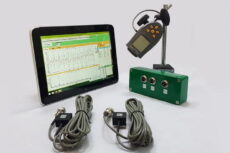
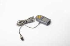
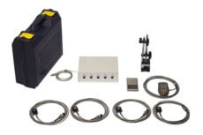
Professional Vibration Analysis Equipment
Identify resonance problems and balance rotors in the field with Vibromera's portable devices — spectrum analysis, phase measurement, and ISO-compliant balancing in one instrument.
Browse Equipment →