Razumevanje N+2 metode u viseravansadbalanasiranju


The N+2 method is an advanced balansiranje procedura korišćena za viseravansadbalansiranje of fleksibilni rotori. Its name comes from a correction-plane rule formalised in ISO 21940-12 (formerly ISO 11342): to balance a rotor through N flexural critical (resonance) speeds when low-speed rigid-body balancing is also carried out, the rotor generally needs N korekcijskih ravnina for the N flexible modes plus two more for the rigid-body (static and couple) unbalance — N+2 planes in total. Do not confuse this with the run count: in the practical influence-coefficient procedure described in this article, N denotes the number of correction planes actually used, and the job then takes N+2 runs — one initial baseline, N trial-weight runs (one for each plane) and a final verification. The method extends the logic of balansiranja u dvije ravnine na rotore koji trebaju tri ili više ravnina, situacija česta u visokobrzinim turbinama, kompresorima, generatorima i dugim valjcima papirnih mašina.
1. Definicija: Što je N+2 metoda
A rigid rotor pokretanja ispod svoje prve critical speed mogu se dovesti u dozvoljene vrijednosti jednostavnom korekcijom u jednoj ili dvije ravnine, jer njihova unbalance distribucija neuravnoteženosti se ne mijenja sa brzinom. Fleksibilni rotor je drugačiji: nakon što se pokretanja pri ili iznad kritične brzine, on se savija, a to savijanje redistribuira efektivnu neuravnoteženost duž njegove dužine. Korekcija zato zahtijeva nekoliko ravnina raspoređenih duž osovine, i metodu koja može raščlaniti kako svaka ravnina utječe na vibracije na svim ostalim mjestima. N+2 metoda je ta sustavna procedura obračuna — disiplinirani način da se rotor u potpunosti karakterizira, a zatim se riješi najbolja korekcija u svakoj ravnini odjednom.
2. Matematička osnova
N+2 metoda je izgrađena na metoda koeficijenata utjecaja, generalizirano sa jedne ili dvije ravnine na mnoge.
Matrica koeficijenata utjecaja
For a rotor with N correction planes and M measurement locations (typically M ≥ N), the system is described by an M×N matrix of influence coefficients. Each coefficient αij prikazuje kako jedinična masa smještena u korekcijskoj ravnini j utječe na vibracije zabilježene na mjestu mjerenja i. Sa četiri korekcijske ravnine i četiri mjesta mjerenja, na primjer:
- α11, α12, α13, α14 opisuju kako svaka od četiri ravnine utječe na mjesto mjerenja 1;
- α21, α22, α23, α24 opisati učinke na mjestu mjerenja 2;
- i tako dalje za mjesta 3 i 4.
To proizvodi matricu 4×4 koja zahtijeva određivanje šesnaest koeficijenata utjecaja. Svaki koeficijent je složena veličina koja nosi i magnitudu i phase kut, jer se odziv rotora zaostaje za primijenjenom silom.
Rješavanje sustava
Kada su svi koeficijenti poznati, softver za uravnoteživanje rješava sustav od M istodobnih vektorskih jednadžbi kako bi pronašao N korekcijskih težina (W1, W2, … Wn) koje minimiziraju vibration na svim M mjestima istovremeno. To se oslanja na vektorsku matematiku i algoritme inverzije matrice (ili metodu najmanjih kvadrata). Kada M premašuje N, sustav je preodrđen i rješenje metodom najmanjih kvadrata pronalazi skup korekcija koji daje najmanju rezidualno vibracije na svim senzorima — robusniji ishod u prisustvu šuma mjerenja.
3. Postupak N+2, korak po korak
Postupak slijedi redoslijed koji se prirodno skalira s brojem korekcijskih ravnina.
Pokus 1 — Mjerenje početne bazne linije
Rotor se vrti brzinom uravnoteživanja u svojem početnom neuravnoteženom stanju. Amplituda vibracija i phase bilježe se na svim M mjestima — obično na svakom leživu, a ponekad i na međuposrednim pozicijama kako bi se uhvatilo gibanje u sredini raspona. Ova mjerenja uspostavljaju vektore početne neuravnoteženosti koji se moraju ispraviti.
Pokusi 2 do N+1 — Sekvencijalni pokusi s ispitnim težinama
Za svaku korekcijsku ravninu redom, od 1 do N:
- Zaustavite rotor i pričvrstite ispitnu težinu poznate mase na poznatu kutnu poziciju samo u toj jednoj ravnini.
- Pokrenite rotor istom brzinom i izmjerite vibracije na svim M mjestima.
- Promjena vibracija — trenutni vektor minus vektorska bazna linija — otkriva kako ta određena ravnina utječe na svako mjesto mjerenja, dajući jedan stupac matrice koeficijenata.
- Uklonite ispitnu težinu prije nego što prijeđete na sljedeću ravninu (osim ako se namjerno primjenjuje varijanta "ostani" kako bi se uštedjeli pokusi).
Nakon svih N pokušajnih pokretanja, poznata je potpuna M×N matrica koeficijenata uticaja.
Faza izračunavanja
Instrument rješava matrične jednačine da bi izračunao tražene tegovi za korekciju — i masu i kut — za svaku od N ravni.
Pokretanje N+2 — Provjera
Sve N izračunate korekcije trajno se instaliraju i finalno pokretanje potvrđuje da je vibracija pala na prihvatljive nivoe na svakom mjestu mjerenja. Ako rezultat još nije zadovoljavajući, trim balance ili se provodi dodatna iteracija koristeći koeficijente koji su već dostupni.
4. Obrađeni primjer: Balansiranje sa četiri ravni (N = 4)
Za dugačak fleksibilan rotor koji zahtijeva četiri ravni korekcije:
- Total runs: 4 + 2 = 6.
- Run 1: početno mjerenje na svim četirima osloncima.
- Run 2: pokušajna težina u ravni 1, mjerenje svih četiriju oslonaca.
- Run 3: pokušajna težina u ravni 2, mjerenje svih četiriju oslonaca.
- Run 4: pokušajna težina u ravni 3, mjerenje svih četiriju oslonaca.
- Run 5: pokušajna težina u ravni 4, mjerenje svih četiriju oslonaca.
- Run 6: provjera sa svim četirima korekcijama instaliranim.
Ovo gradi 4×4 matricu od šesnaest koeficijenata, koja se rješava da bi se pronašle četiri optimalne težine korekcije. Ista aritmetika za jednostavniji posao je dio kalkulator koeficijenata uticaja, koji rješava slučaj sa jednom ravni i čini temeljnu vektorsku metodu lako vidljivom prije skaliranja.
5. Prednosti N+2 metode
Ovaj pristup nudi nekoliko važnih prednosti za rad sa više ravni:
- Sistematično i potpuno: svaka korekcijska ravnina se testira nezavisno, što daje potpunu karakterizaciju sistema rotor-ležaja‘s odgovora kroz sve ravnine i lokacije.
- Hvata kompleksne unakrsne sprege: na fleksibilnim rotorimase težina u bilo kojoj ravnini može uticati na vibracije na svakom ležaju; matrica eksplicitno beleži sve te interakcije.
- Matematički rigorozan: koristi dobro uspostavljene tehnike linearne algebre (matrična inverzija, prilagođavanje najmanjim kvadratima) koje daju optimalna rešenja kada se sistem ponaša linearno.
- Fleksibilna strategija merenja: dozvoljavanje da M premaši N proizvodi predeterminisani sistem koji je otporniji na šum.
- Industrijski standard za kompleksne rotore: to je prihvaćena metoda za brzohodnu turbomašineriju i druge kritične aplikacije sa fleksibilnim rotorima.
6. Izazovi i ograničenja
Uravnotežavanje više ravnina metodom N+2 takođe predstavlja pravi izazov:
- Povećana složenost: broj test-pokretanja raste linearno sa brojem ravnina. Uravnotežavanje sa šest ravnina zahteva osam pokretanja, što oštrо povećava vremenske gube, troškove i habanje mašine.
- Zahtevi za tačnošću merenja: rešavanje velikih matrica pojačava efekat greške merenja, pa su neophodna visokokvalitetna instrumentacija i pažljiva tehnika.
- Numerička stabilnost: matrična inverzija može postati loše uslovljena kada su korekcijske ravnine previše bliske, kada izabrane lokacije merenja ne uspevaju da zabeleze odgovore rotora, ili kada test-težine proizvode samo marginalne promene vibracija.
- Time and cost: svaka dodatna ravnina dodaje još jedno pokretanje, produžavajući zastoje i rad; za kritičnu opremu to mora biti procenjeno nasuprot dobitka u kvalitetu uravnotežavanja.
- Zahtijeva napredni softver: rješavanje N×N sistema kompleksnih vektorskih jednadžbi daleko je izvan mogućnosti ručnog izračunavanja, pa je specijalizirani softver za uravnotežavanje više ravni obavezatan.
7. Kada koristiti N+2 metodu
Metoda je primjena kada:
- rotor je stvarno fleksibilan: radi iznad svoje prve — i eventualno druge ili treće — critical speed.
- rotor je dug i štitav: veliki omjer dužine i promjera znači značajno savijanje vratila u radu.
- Uravnotežavanje dva ravni je dokazano nedostatno: earlier two-plane pokušaji nisu uspjeli postići prihvatljiv rezultat.
- Više kritičnih brzina mora se prijeći tijekom normalnog rada.
- Oprema je visoke vrijednosti: kritične turbine, kompresori ili generatori gdje je sveobuhvatno uravnotežavanje opravdano.
- Vibracija je intenzivna na međuposrednim mjestima, između krajnjih ležajeva, signalizirajući neuravnoteženost srednje grede koju ispravka krajnjih ravni ne može dosegnuti.
8. Alternativa: Modalno uravnotežavanje
Za najfleksibilnije rotore, modalno uravnotežavanje može biti bolje od konvencionalnog N+2 pristupa. Umjesto minimiziranja vibracija na specifičnim brzinama, modalno uravnotežavanje ciljanja specifičnih moda vibracija jedan po jedan, iskorištavajući mode shapes postići rezultat s manje pokusnih pokretanja. Kompromis je što zahtijeva još dublje razumijevanje rotor dynamics i napredniju analizu. U praksi se obje filozofije često kombiniraju — modalna analiza vodi gdje ravnine idu, a rješenje s koeficijentima utjecaja dorađuje mase.
9. Najbolja praksa za uspjeh
Planning
- Pažljivo odaberite N lokacija korekcijskih ravnina — dobro razmaknute, dostupne, idealno poravnate s oblikom moda rotora antinodes, jer uteg postavljen u čvoru ima malo utjecaja na taj mod.
- Odaberite M ≥ N mjesta mjerenja koja u dostatnoj mjeri hvataće vibracijsko ponašanje rotora.
- Planirajtevrijeme za toplinsku stabilizaciju između pokretanja.
- Pripremite pokusne utege i instalacijski hardver unaprijed.
Execution
- Održavajte radne uvjete — brzinu, temperaturu, opterećenje — apsolutno konzistentno kroz svih N+2 pokretanja.
- Koristite pokusne utege dovoljno velike da proizvedu jasan, mjerljiv odgovvor, tipično promjenu vibracije od 25–50%.
- Izvršite nekoliko mjerenja po pokretanju i prosječite ih kako biste potisnuli šum.
- Dokumentirajte masu, kut i radius svakog pokusnog utega.
- Provjerite kvalitetu mjerenja faze, jer se greške faze pojačavaju u velikim matričnim rješenjima.
Analysis
- Pregledajte matricu koeficijenata utjecaja radi anomalija ili neočekivanih obrazaca.
- Provjerite broj uvjetovanosti matrice — visoke vrijednosti upozoravanje numeričke nestabilnosti.
- Potvrdite da su izračunate korekcije fizički razumne, niti pretjerano velike niti zanemarljivo male.
- RazmotriteSimulaciju očekivanog konačnog rezultata prije nego što se korekcije primijene.
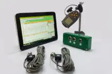
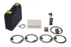
10. Praktična primjena na terenu i Balanset-1A
Većina balansiranja fleksibilnih rotora na kritičnim strojevima vrši se na mjestu pri radnoj brzini, gdje se rotor zapravo savija, a ne na stroju za balansiranje s niskom brzinom. Prijenosni dvokanalani analizator kao što je Balanset-1A pruža građivne blokove koje metoda N+2 trebam: sinhronizirana mjerenja amplitude i faze 1× na svakom ležaju, automatski proračun koeficijenata utjecaja iz pokusnih pokretanja s utegom, i potvrda rezidualnu neuravnoteženost nakon što su ispravke instalirane. Za trosjedinjene balansiranja instrument direktno provodi potpuno rješenje matrice utjecaja; za veće broj ravnina njegovi su jednoravljsni i dvosjedinjeni mjerenja disciplinirani po-ravninski podaci koje višesjedinjeni rješavač kombinira. Budući da se rad odvija u sopstvenim ležajevima mašine, snimljena odziva uključuje realnu krutost oslonca i termičko stanje u kojem se rotor nalazi.
11. Integracija s drugim tehninama
Metoda N+2 može se kombinirati s komplementarnim pristupima:
- Balansiranje s promjenom brzine: ponovite mjerenja N+2 na nekoliko brzina kako biste optimizirali balans u cijelom radnom opsegu, a ne samo na jednoj brzini.
- Hibridni modalni–konvencionalni: use modal analysis kako biste obavijestili izbor ispravne ravnine, zatim primijenite metodu N+2 da odredite veličine težina.
- Iterativno usavršavanje: izvršite potpuno balansiranje N+2, zatim ponovno koristite reducirani skup koeficijenata utjecaja za brzo trim balancing kako se uvjeti mijenjaju tijekom rada.
