The Time Waveform: The Foundation of Vibration Analysis


The time waveform — also called the time-domain signal — is the raw, unprocessed signal that comes straight from a vibration transducer such as an accelerometer or a proximity probe. It is a graph that plots the instantaneous amplitude of the vibration on the vertical (Y) axis against time on the horizontal (X) axis. In other words, it is a direct, moment-by-moment picture of the physical back-and-forth movement of the machine at the sensor location over a short window of time — the original record from which every other view of the data is derived.
1. Definition: What is a Time Waveform?
Before any mathematical processing, the sensor produces a continuously varying voltage proportional to motion. When that voltage is sampled and displayed against time, the result is the time waveform. It is the most literal representation of vibration there is: nothing has been averaged, filtered or transformed away. Every other tool an analyst uses — the spectrum, statistical indicators, orbit plots — is computed from this signal, which is why understanding the waveform underpins all of vibration analysis.
Because it preserves the true sequence of events, the waveform answers a question the frequency domain cannot: not just which frequencies are present, but exactly when and how hard each event struck.
2. The Role of the Time Waveform in Diagnostics
While the frequency spectrum (FFT) is the primary tool for diagnosing most steady-state machinery faults, the time waveform is an indispensable and complementary partner. The FFT calculates the frequency content averaged over the duration of the sample, and in doing so it can blur or hide short-duration, transient or non-periodic events. The waveform shows exactly what happened from one instant to the next, which makes it superior for analysing:
- Impulsive events: it clearly shows the sharp impacts that are often the first sign of bearing or gear defects.
- Modulation and beats: the classic rise-and-fall pattern of beating is most clearly seen in the time waveform.
- Transient events: it can capture random, one-off events that an FFT would simply average out.
- Signal clipping: it immediately reveals if the sensor signal has exceeded the analyser’s input range — a condition that would invalidate the FFT entirely.
- Rubs: the sharp, distorted signature of a rotor rub is often most obvious in the waveform.
For this reason a skilled analyst always reviews both the spectrum and the time waveform together; relying on either one alone leaves part of the machine’s story untold.
3. How to Analyse a Time Waveform
Reading a waveform means examining its shape and a handful of key characteristics. The settings used to capture it matter too — the sample length must be long enough to contain several revolutions of the shaft, and the sampling rate high enough to avoid aliasing of the high-frequency content that impacts produce.
Peak Amplitude
The maximum amplitude — the peak — is a direct measure of the largest force or stress in an event. A high peak sitting in an otherwise low-energy signal is a strong indicator of impacting. Because impacts are so brief, analysts often look at the true peak rather than a smoothed value, and may quote it peak-to-peak for displacement signals.
Overall Shape
A healthy, well-balanced machine usually produces a clean, sinusoidal waveform at the running-speed frequency. Distortions of that shape reveal the presence of other frequencies or forces. A “flattened” or “clipped” appearance, for example, is a classic sign of mechanical looseness, where the component’s motion is being physically constrained at the extremes of travel.
Repetitive Patterns and Periodicity
By placing cursors on the plot an analyst can measure the time between repeating events:
- The time between major peaks gives the period of the fundamental vibration, which inverts directly into its frequency (Frequency = 1 / Period).
- Smaller, repetitive impacts “riding” on the main waveform can pin down the precise repetition rate of a bearing or gear fault — often before that fault is clearly visible in the spectrum.
Statistical Parameters
Values calculated from the waveform are powerful, compact diagnostic indicators:
- RMS (Root Mean Square): measures the overall energy content of the signal and tracks general severity.
- Crest Factor: the ratio of peak amplitude to RMS. A high crest factor (well above 3) signals strong impacting against an otherwise modest energy level.
- Kurtosis: a measure of the “peakedness” of the signal that is highly sensitive to early-stage bearing faults, often rising before RMS does.
4. Capturing the Waveform in the Field
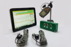
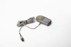
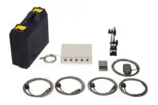
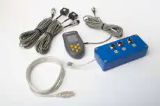
A waveform is only useful if it is captured cleanly on the running machine. A portable two-channel instrument such as the Balanset-1A records the raw time-domain signal from its accelerometers alongside the FFT spectrum, so the analyst can switch between the two views of the same measurement on site. Seeing the live waveform while the machine runs makes it immediately obvious whether the signal is clipping, whether sharp impacts are present, and whether the captured window is long and steady enough to trust — checks that are far harder to make from a processed spectrum alone.
5. Waveform vs. Spectrum: A Partnership
The time waveform and the frequency spectrum are two different views of the same data, and they work best in combination rather than competition:
- The spectrum excels at separating multiple, closely spaced, steady-state frequencies — for instance distinguishing running-speed harmonics from a nearby gear-mesh component.
- The waveform excels at revealing the true amplitude of impacts and the nature of non-steady-state events.
A common example makes the partnership concrete: the spectrum might show only a slightly raised noise floor, while the waveform reveals that the cause is a train of low-amplitude, repetitive impacts from a developing bearing fault. One view flags that something has changed; the other explains what it is. Together they give the complete picture of machine health.