ಮುನ್ಸೂಚಕ ನಿರ್ವಹಣೆಯಲ್ಲಿ ರೋಗನಿರ್ಣಯವನ್ನು ಅರ್ಥಮಾಡಿಕೊಳ್ಳುವುದು


ಪೂರ್ವಾನುಮಾನ (ಅಸಫಲತೆ ಮುನ್ನೋಡು ಎಂದೂ ಕರೆಯುತ್ತಾರೆ, ಮತ್ತು ನಿಕಟವಾಗಿ ಸಂಬಂಧಿತವಾಗಿದೆ ಉಳಿದ-ಉಪಯುಕ್ತ-ಆಯುಷ್ಯ ಅಂದಾಜು) ಎಂಬುದು ಪತ್ತೆಯಾದ ದೋಷವು ಕಾರ್ಯನಿರತ ವೈಫಲ್ಯತೆ ಅಥವಾ ಹಸ್ತಕ್ಷೇಪದ ಬೇಡಿಕೆಯನ್ನು ಉಂಟುಮಾಡುವ ಮೊದಲು ಎಷ್ಟು ಸಮಯ ಉಳಿದಿದೆ ಎಂಬುದನ್ನು ನಿರ್ಣಯಿಸುವ ಪ್ರಕ್ರಿಯೆ. ರೋಗನಿರ್ಣಯವು ಧರಣಾಪೂರ್ವಣ (ಸಮಸ್ಯೆ ಇದೆ ಎಂದು ತಿಳಿಯುವುದು) ಮತ್ತು ರೋಗನಿರ್ಣಯ (ಸಮಸ್ಯೆ ಏನೆಂದು ತಿಳಿಯುವುದು), ಮತ್ತು ನಿರ್ಣಾಯಕ ಪ್ರಶ್ನೆಗೆ ಉತ್ತರ ನೀಡುತ್ತದೆ — “ನಾವು ಯಾವಾಗ ಕ್ರಮ ತೆಗೆದುಕೊಳ್ಳಬೇಕು?” — ವಿಶ್ಲೇಷಿಸುವ ಮೂಲಕ vibration ಪ್ರಗತಿ ಪ್ರವೃತ್ತಿಗಳು, ದೋಷ ಪ್ರಕಾರದ ಗುಣಲಕ್ಷಣಗಳು, ಮತ್ತು ಯಂತ್ರದ ಕಾರ್ಯಾಚರಣಾ ಪರಿಸ್ಥಿತಿಗಳು.
ನಿಖರವಾದ ಮುನ್ಸೂಚನೆಯು ಏನನ್ನು ಮಾಡುತ್ತದೆ ಭವಿಷ್ಯದ ನಿರ್ವಹಣೆ ನಿಜವಾಗಿಯೂ ಪೂರ್ವಾನುಮಾನಾತ್ಮಕ. ಇದು ಶ್ರೇಷ್ಠ ಕ್ಷಣದಲ್ಲಿ ನಿರ್ವಹಣೆಯನ್ನು ನಿಗದಿಪಡಿಸಲು ಅನುಮತಿ ನೀಡುತ್ತದೆ — ತುಂಬಾ ಶೀಘ್ರವಾಗಿ ಅಲ್ಲ, ಇದು ಉಳಿದ ಜೀವನವನ್ನು ವ್ಯರ್ಥ ಮಾಡುತ್ತದೆ, ಅಥವಾ ತುಂಬಾ ತಡವಾಗಿ ಅಲ್ಲ, ಇದು ವಿಫಲತೆಗೆ ಕಾರಣವಾಗುತ್ತದೆ — ಮತ್ತು ಇದು ದೀರ್ಘ-ಸೀಸೆ ಸ್ಪೇರ್ಗಳ ಸಂಗ್ರಹ, ಶ್ರಮ ಮತ್ತು ಉಪಕರಣಗಳ ಹಂಚಿಕೆ, ಮತ್ತು ಉತ್ಪಾದನೆಯ ಸಮನ್ವಯವನ್ನು ಆಧಾರಒಣ್ಣಿಸುತ್ತದೆ. ವ್ಯಾಪಕ ಯೋಜನೆಯೊಳಗೆ ಸ್ಥಿತಿ-ಆಧಾರಿತ ನಿರ್ವಹಣೆ, ಮುನ್ಸೂಚನೆಯು ಮುಂದಕ್ಕೆ ನೋಡುವ ಹಂತವಾಗಿದೆ ಇದು “ಈ ಯಂತ್ರವು ರೋಗಿ”ನಿಂದ “ಈ ಯಂತ್ರವನ್ನು ಎಂಟನೇ ವಾರದ ಮೂಲಕ ಸರಿಪಡಿಸಬೇಕು.”ಗೆ ತಿರುಗಿಸುತ್ತದೆ
1. ಮೂರು-ಹಂತದ ಸರಪಳಿ: ಸನ್ನಿವೇಶ, ರೋಗನಿರ್ಣಯ, ಮುನ್ಸೂಚನೆ
ಮುನ್ಸೂಚನೆಯನ್ನು ಸರಪಳಿಯೊಳಗಿನ ಮೂರನೇ ಸಂಪರ್ಕವಾಗಿ ನೋಡಲು ಇದು ಸಹಾಯ ಮಾಡುತ್ತದೆ. ಪತ್ತೆಹಚ್ಚಿಕೆ ಒಂದು ಪ್ರಾಚಲವು ಅದರ ಬಾಹ್ಯ ಭಾಗವನ್ನು ಗಮನಿಸುತ್ತದೆ baseline. ನಿರ್ಣಯ ಕಾರ್ಯವಿಧಾನವನ್ನು ಗುರುತಿಸುತ್ತದೆ — ಎ ಬೇರಿಂಗ್ ದೋಷ, misalignment, ಸಡಿಲತೆ. ಪೂರ್ವಾನುಮಾನ ತದನಂತರ ಆ ಕಾರ್ಯವಿಧಾನವನ್ನು ಸಮಯಕ್ಕೆ ಮುಂದೆ ಪ್ರಕ್ಷೇಪಿಸುತ್ತದೆ. ಪ್ರತಿಯೊಂದು ಹಂತವು ಅದರ ಮೊದಲನೆಯ ಮೇಲೆ ಅವಲಂಬಿತವಾಗಿರುತ್ತದೆ: ನೀವು ಸರಿಯಾಗಿ ಹೆಸರಿಸದಿರುವ ದೋಷದ ಭವಿಷ್ಯತ್ತವನ್ನು ಊಹಾ ಮಾಡಲು ಸಾಧ್ಯವಾಗುವುದಿಲ್ಲ, ಅದಕ್ಕಾಗಿಯೇ ಆತ್ಮವಿಶ್ವಾಸಯುತ ರೋಗನಿರ್ಣಯವು ಯಾವುದೇ ನಿರ್ಭರ ಪ್ರವಚನದ ಅಡಿಪಾಯವಾಗಿದೆ. ಸಂಪೂರ್ಣ ಸರಪಳಿಯನ್ನು ಮೇಲ್ವಿವರಣೆ ಮಾನದಂಡಗಳಲ್ಲಿ ಔಪಚಾರಿಕಗೊಳಿಸಲಾಗಿದೆ ಅಂದರೆ ISO 13374, ಇದು ಸನ್ನಿವೇಶ, ರೋಗನಿರ್ಣಯ, ಮತ್ತು ಮುನ್ಸೂಚನೆಯನ್ನು ವಿಭಿನ್ನ ಡೇಟಾ-ಪ್ರಕ್ರಿಯೆಗೊಳಿಸುವ ಕಾರ್ಯಗಳಾಗಿ ಹೊರತೆಗೆಯುತ್ತದೆ.
2. ಮುನ್ಸೂಚನೆ ವಿಧಾನಗಳು
ಪ್ರವೃತ್ತಿ ಹೊರತೆಗೆಯುವಿಕೆ
ಅತ್ಯಂತ ಸಾಮಾನ್ಯ ಮತ್ತು ಪ್ರಾಯೋಗಿಕ ವಿಧಾನ, ಮತ್ತು ದೈನಿಕ ವಿಸ್ತರಣೆ ಪ್ರವೃತ್ತಿ ವಿಶ್ಲೇಷಣೆ:
- ಸಮಯದ ವಿರುದ್ಧ ಐತಿಹಾಸಿಕ ಕಂಪನ ಡೇಟಾವನ್ನು ರೂಪಿಸಿ.
- ಒಂದು ಪ್ರವೃತ್ತಿ ರೇಖೆ ಅಳವಡಿಸಿ — ರೇಖೀಯ, ಘಾತೀಯ, ಅಥವಾ ಬೇರೆ ರೀತಿಯ.
- ಎಚ್ಚರಿಕೆ ಅಥವಾ ವಿಫಲತೆ ಎಂದು ಕಂಡುಹಿಡಿಯಲು ಹೊರತೆಗೆಯಿರಿ ಮಿತಿ ಮೌಲ್ಯ ಅತಿಕ್ರಮಿಸಲ್ಪಡುವ ಸಮಯವನ್ನು ಊಹಿಸಲು.
- ಪ್ರತಿಯೊಂದು ಹೊಸ ಮಾಪನದೊಂದಿಗೆ ಮುನ್ಸೂಚನೆಯನ್ನು ನವೀಕರಿಸಿ.
- ನಿಖರತೆ: ಮಧ್ಯಮ (ಇದು ಪ್ರವೃತ್ತಿ ಮುಂದುವರಿಯುತ್ತದೆ ಎಂದು ಭಾವಿಸುತ್ತದೆ).
- ಅವಶ್ಯಕತೆಗಳು: ಸಾಕಷ್ಟು ಪ್ರವೃತ್ತಿ ಇತಿಹಾಸ — ಕನಿಷ್ಠ ಆರು ಡೇಟಾ ಪಾಯಿಂಟ್ಗಳು.
ಭೌತಿಕ ವಿದ್ಯೆ-ಆಧಾರಿತ ಮಾದರಿಗಳು
- ವಿಫಲತೆ ಭೌತಿಕತತ್ವದ (ಬಿರುಕು ಬೃದ್ಧಿ, ಸ್ಪಾಲ್ ಪ್ರಸರಣ) ತಿಳುವಳಿಕೆಯ ಮೇಲೆ ನಿರ್ಮಿತ.
- ಮಾದರಿ ಒತ್ತಡ, ಚಕ್ರ ಮತ್ತು ಪರಿಸರದಿಂದ ಪ್ರಗತಿ ಭವಿಷ್ಯದ್ವಾಣಿ ಮಾಡುತ್ತದೆ.
- ಉದಾಹರಣೆಗಳು: ಬಿರುಕು ಬೃದ್ಧಿಗೆ ಪ್ಯಾರಿಸ್ ನಿಯಮ, ಅಥವಾ ಬೇರಿಂಗ್ L10 ಆಯುಷ್ಯ-ಲೆಕ್ಕಾಚಾರಗಳನ್ನು ಚೋರ್ನೀಕರಿಸು.
- ನಿಖರತೆ: ಉತ್ತಮ, ಮಾದರಿ ನಿಯತಾಂಕಗಳು ತಿಳಿದಿದ್ದಾಗ.
- ಅವಶ್ಯಕತೆಗಳು: ವಿವರವಾದ ಸಾಧನ ಮತ್ತು ಕಾರ್ಯಾಚರಣ ಡೇಟಾ.
ಅನುಭವ-ಆಧಾರಿತ (ಐತಿಹಾಸಿಕ ಡೇಟಾ)
- ಇದೇ ರೀತಿಯ ಸಾಧನಗಳ ಹಿಂದಿನ ವಿಫಲತೆಗಳ ಮೇಲೆ ನಿರ್ಮಿತ.
- ಇತಿಹಾಸದಿಂದ ಸೆಳೆಯಲಾದ ವಿಶಿಷ್ಟ ಪ್ರಗತಿ ದರಗಳನ್ನು ಬಳಸುತ್ತದೆ.
- ಅನುಭವಾತ್ಮಕ ಸಂಬಂಧಗಳ ಮೇಲೆ ಅವಲಂಬನೀಯ (ಕಂಪನ ಮಟ್ಟ → ವಿಫಲತೆಗೆ ಸಮಯ).
- ನಿಖರತೆ: ನ್ಯಾಯ, ಮತ್ತು ಸಾಧನ-ನಿರ್ದಿಷ್ಟ.
- ಅವಶ್ಯಕತೆಗಳು: ಐತಿಹಾಸಿಕ ವಿಫಲತೆ ಡೇಟಾಬೇಸ್.
ಅಂಕಿ ಅಂಶ / ಯಂತ್ರ ಕಲನೆ
- ಐತಿಹಾಸಿಕ ಪ್ರಗತಿ ಡೇಟಾದಲ್ಲಿ ತರಬೇತಿ ಪಡೆದ ಕ್ರಮಾವಳಿಗಳು.
- ಅನೇಕ ಇದೇ ಪ್ರಕರಣಗಳಲ್ಲಿ ಮಾದರಿ ಸ್ವೀಕೃತಿ.
- ಸಂಭವನೀಯ ಭವಿಷ್ಯದ್ವಾಣಿಗಳನ್ನು ಉತ್ಪಾದಿಸುತ್ತದೆ.
- ನಿಖರತೆ: ಸಾಕಷ್ಟು ಡೇಟಾ ಇದ್ದರೆ ಸಂಭಾವ್ಯ ಅತ್ಯಂತ ಉತ್ತಮ.
- ಅವಶ್ಯಕತೆಗಳು: ದೊಡ್ಡ ಡೇಟಾಸೆಟ್ ಮತ್ತು ಕಂಪ್ಯೂಟೇಶನಲ್ ಸಂಪನ್ಮೂಲಗಳು.
3. ಮುನ್ನರೋಜನೆಯ ನಿಖುಂತತೆಯನ್ನು ಪ್ರಭಾವಿಸುವ ಅಂಶಗಳು
ಟ್ರೆಂಡ್ ಡೇಟಾ ಗುಣಮಾನ
- ಹೆಚ್ಚು ಡೇಟಾ ಬಿಂದುಗಳು ಟ್ರೆಂಡ್ ವ್ಯಾಖ್ಯಾನವನ್ನು ತೀಕ್ಷ್ಣವಾಗಿ ಮಾಡುತ್ತವೆ.
- ಸುಸಂಗತ ಮಾಪನಗಳು ವಿಶ್ವಾಸಾರ್ಹ ಟ್ರೆಂಡ್ಗಳನ್ನು ಮೆಲುವು.
- ಸಾಕಷ್ಟು ಇತಿಹಾಸ (ಕನಿಷ್ಠ ತಿಂಗಳುಗಳು) ಅತ್ಯಗತ್ಯ.
- ಸ್ವಚ್ಛ ಡೇಟಾ, ಬಾಹ್ಯಮುಖಗಳನ್ನು ಗುರುತಿಸಿದ್ದೆ, ನಿರಾಳ ಹಾಗಿಮೂಲೆಗಳನ್ನು ತಡೆಯುತ್ತದೆ.
ದೋಷ ಪ್ರಗತಿ ಗುಣಲಕ್ಷಣಗಳು
- ಮುನ್ನೆಳೆಯಬಹುದಾದ ಪ್ರಗತಿ: ಮುನ್ನರೋಜಿಸುವುದು ಸುಲಭ — ಉದಾಹರಣೆಗೆ ಹೆಚ್ಚುವರಿ ಬೇರಿಂಗ್ ಧರಣೆ.
- ವೇಗವರ್ಧಕ ಪ್ರಗತಿ: ಕಷ್ಟಕರ — ಸ್ಪಾಲ್ ಬೆಳವಣಿಗೆ ಸರಿಸುಮಾರು ವಿಸರ್ಜಿತ.
- ಅನಿಯಮಿತ ಪ್ರಗತಿ: ಕಠಿಣ — ಸಡಿಲಿಕೆ ಮತ್ತು ಸಂಭ್ರಮಾಪೂರ್ಣ ರಬ್ಬಿಂಗ್ಗಳು.
- ಹಠಾತ್ ವೈಫಲ್ಯ: ಮೂಲಭೂತವಾಗಿ ಅನಿರೀಕ್ಷಿತ — ಶಾಫ್ಟ್ ತುಂಡುಮುಂಡಾಗುವುದರಿಂದ ಬಿರುಕು.
ಆಪರೇಟಿಂಗ್ ಸ್ಥಿತಿ ಸ್ಥಿರತೆ
- ಸ್ಥಿರ ಸ್ಥಿತಿಗಳು ವಿಶ್ವಾಸಾರ್ಹ ಮುನ್ನರೋಜನೆಗಳನ್ನು ಬೆಂಬಲಿಸುತ್ತವೆ.
- ವೇರಿಯಬಲ್ ಲೋಡ್ಗಳು ಮತ್ತು ವೇಗಗಳು ಮುನ್ನರೋಜನೆಗಳನ್ನು ಕಡಿಮೆ ಖಚಿತವಾಗಿ ಮಾಡುತ್ತವೆ.
- ಪ್ರಕ್ರಿಯೆ ಬದಲಾವಣೆಗಳು ಪ್ರಗತಿಯನ್ನು ವೇಗವರ್ಧಿಸುವ ಅಥವಾ ನಿಧಾನ ಮಾಡುವ ಸಾಧ್ಯತೆ ಇದೆ.
4. ಉಳಿದ ಉಪಯುಕ್ತ ಜೀವನ (RUL) ಮತ್ತೆ ಅಂದಾಜು
ಪ್ರಾಗ್ನೋಸಿಸ್ನ ಪ್ರಮುಖ ಔಟ್ಪುಟ್ ಆಗಿದೆ ಉಳಿದ ಉಪಯುಕ್ತ ಜೀವನ: ಪ್ರಸ್ತುತ ಸ್ಥಿತಿಯಿಂದ ವೈಫಲ್ಯ ಅಥವಾ ಮಧ್ಯಸ್ಥ ಮಾನದಂಡಕ್ಕೆ ಬರುವ ಸಮಯ।
ಇದನ್ನು ಹೇಗೆ ವ್ಯಕ್ತ ಮಾಡಲಾಗುತ್ತದೆ
- ಕಾರ್ಯಾಚರಣಾ ಘಂಟೆಗಳು, ಕ್ಯಾಲೆಂಡರ್ ದಿನಗಳು ಅಥವಾ ಚಕ್ರಗಳಲ್ಲಿ ಮಧ್ಯಸ್ಥ ಅಗತ್ಯವಾಗುವವರೆಗೆ ತಿಳಿಸಲಾಗುತ್ತದೆ।
- ಹೊಸ ಡೇಟಾ ಆಗಮನದೊಂದಿಗೆ ನಿರಂತರವಾಗಿ ನವೀಕರಣ ಮಾಡಲಾಗುತ್ತದೆ।
- ನಿಜವಾದ ಅನಿಶ್ಚಿತತೆಯನ್ನು ಹೊಂದಿರುವ ಅಂದಾಜುಾಗಿ ವರದಿ ಮಾಡಲಾಗುತ್ತದೆ।
ಆತ್ಮವಿಶ್ವಾಸ ಮಾರ್ಜಿನ್ಗಳು
- RUL ಒಂದು ಅಂದಾಜು, ಸತ್ಯವಲ್ಲ।
- ಶ್ರೇಷ್ಠವಾಗಿ ಒಂದು ವ್ಯಾಪ್ತಿಯಾಗಿ ವ್ಯಕ್ತಪಡಿಸಲಾಗುತ್ತದೆ — ಉದಾಹರಣೆಗೆ “30–90 ದಿನಗಳು 90% ನಿಶ್ಚಿತತೆಯೊಂದಿಗೆ।”
- ವೈಫಲ್ಯ ಹತ್ತಿರವಾಗುತ್ತಿದ್ದಂತೆ ಮತ್ತು ಹೆಚ್ಚಿನ ಡೇಟಾ ಸಂಗ್ರಹವಾದಂತೆ ಅನಿಶ್ಚಿತತೆ ಕುಗ್ಗುತ್ತದೆ।
- ಸಂವೇದನಶೀಲ ಅಂದಾಜುಗಳು ಸೂಕ್ತವಾಗಿವೆ ನಿರ್ಣಾಯಕ ಯಂತ್ರೋಪಕರಣ.
ಕಾರ್ಯಾತ್ಮಕ ಉದಾಹರಣೆ
- ಬೇರಿಂಗ್ ದೋಷ 2 g ನಲ್ಲಿ ಸೂಚಿಸಲಾಗುತ್ತದೆ ಎನ್ವೆಲಪ್ ಆಂಪ್ಲಿಟ್ಯೂಡ್.
- ಐತಿಹಾಸಿಕ ಪ್ರಗತಿ: 2 g → 10 g (ಅಲಾರ್ಮ್ ಮಟ್ಟ) ವಿಶಿಷ್ಟ 60 ದಿನಗಳಲ್ಲಿ।
- ಪ್ರಸ್ತುತ ಪ್ರವಾಹ: ಸ್ವಲ್ಪ 0.5 g ಪ್ರತಿ ವಾರ ಹೆಚ್ಚುತ್ತಿವೆ।
- ಪೂರ್ವಾಭಾಸ: ಅಲಾರ್ಮ್ ಮಟ್ಟವನ್ನು ಸರಿಸುಮಾರು 10 ವಾರಗಳಲ್ಲಿ ಮೀರಲಾಗುವುದು।
- ಶಿಫಾರಸು: 6–8 ವಾರಗಳ ಒಳಗೆ ನಿರ್ವಹಣೆ ಅವಧಿ ನೆಲಸಿಕೊಳ್ಳಿ।
ಆ ಗಣಿತ — ಢಾಲ ಫಿಟ್ ಮಾಡುವುದು ಮತ್ತು ಮಿತಿಗೆ ಪ್ರಕ್ಷೇಪಿಸುವುದು — ಕೃತ್ಯವಾಗಿ ಅದೇ ಒಂದು ವೈಬ್ರೇಶನ್ ಟ್ರೆಂಡ್ ಇಂದ RUL ಎಸ್ಟಿಮೇಟರ್ ಸ್ವಯಂಚಾಲಿತಗೊಳಿಸುತ್ತದೆ, ಮತ್ತು ISO 13381 ಅನುಸರಿಸುವ ಹೆಚ್ಚು ಔಪಚಾರಿಕ ಚಿಕಿತ್ಸೆ ಲಭ್ಯವಾಗಿರುತ್ತದೆ RUL ಪ್ರೋಗ್ನೋಸ್ಟಿಕ್ಸ್ ಕ್ಯಾಲ್ಕುಲೇಟರ್.
5. ಅನ್ವಯಗಳು
ನಿರ್ವಹಣೆ ಶ್ರೇಣಿಯ ಯೋಜನೆ
- RUL ಸೂಚಿಸುವ ಸೂಕ್ತ ಸಮಯದಲ್ಲಿ ನಿಲುಗಡೆಯನ್ನು ಯೋಜಿಸಿ.
- ಉತ್ಪಾದನ ವೇಳಾಪಟ್ಟಿಗಳೊಂದಿಗೆ ಸಂಘಟಿತಗೊಳಿಸಿ.
- ಒಟ್ಟು ಕೆಳಗೇರುವ ಸಮಯವನ್ನು ಕಡಿಮೆ ಮಾಡಲು ಮೆರುಗೆಯನ್ನು ಗುಂಪುಮಾಡಿ.
- ಯಾವುದೇ ಮುಂಚಿತ ಅಥವಾ ತಡವಾದ ಹಸ್ತಕ್ಷೇಪವನ್ನು ತಪ್ಪಿಸಿ.
ಭಾಗಗಳ ನಿರ್ವಹಣೆ
- ಸರಿಯಾದ ನೆಟ್ಟಗೆ ಸಮಯದೊಂದಿಗೆ ಬದಲಿ ಭಾಗಗಳನ್ನು ಆದೇಶಿಸಿ.
- ತುರ್ತು ಪ್ರೇಷಣೆ ವೆಚ್ಚಗಳನ್ನು ತಪ್ಪಿಸಿ.
- ಸುರಕ್ಷತೆ-ಭಾಗಧಾರಣ ಅವಶ್ಯಕತೆಗಳನ್ನು ಕಡಿಮೆ ಮಾಡಿ.
- ಭವಿಷ್ಯದ್ವಾಣಿಯಿಂದ ನಿರ್ದೇಶಿತ ಸಮಯೋಪಯೋಗಿ ವಿತರಣೆ ಸಿದ್ಧತೆ.
ಸಂಪನ್ಮೂಲ ಹಂಚಿಕೆ
- ಹೀಗೆ ಶ್ರಾಪಿತವಾಗುತ್ತಿರುವ ಹಲವಾರು ಯಂತ್ರಗಳಲ್ಲಿ ಆದ್ಯತೆ ನೀಡಿ.
- ಸೀಮಿತ ಸಂಪನ್ಮೂಲಗಳನ್ನು ಅತ್ಯಂತ ತುರ್ತು ಅವಶ್ಯಕತೆಗಳಿಗೆ ನಿರ್ದೇಶಿತ ಮಾಡಿ.
- ಕಾರ್ಮಿಕ ನಿಯೋಜನೆ ಮತ್ತು ಸರಞ್ಜಾಮ ಹಂತನಿರ್ವಹಣೆಯನ್ನು ಮುಂಚಿತವಾಗಿ ಯೋಜಿಸಿ.
6. ಸವಾಲುಗಳು ಮತ್ತು ಸೀಮಿತತೆಗಳು
ಭವಿಷ್ಯದ್ವಾಣಿ ಅನಿಶ್ಚಿತತೆ
- ಗುರುತು ಪ್ರವೃದ್ಧಿ ಎಂದಿಗೂ ಪೂರ್ಣವಾಗಿ ಮುನ್ನಡೆಸಬಹುದಲ್ಲ.
- ಚಾಲನ ಪರಿಸ್ಥಿತಿಗಳು ಎಚ್ಚರಿಕೆಯಿಲ್ಲದೆ ಬದಲಾಗಬಹುದು.
- ಅನಿರೀಕ್ಷಿತ ವರ್ಧನೆಗಳು ಯಾವಾಗಲೂ ಸಾಧ್ಯವಿದೆ.
- ಸುರಕ್ಷತೆ ಮಾರ್ಜಿನ್ಗಳನ್ನು ಸಾಮಾನ್ಯ ಅಭ್ಯಾಸಗಳಾಗಿ ನಿರ್ವಹಿಸಿ.
ಡೇಟಾ ಅವಶ್ಯಕತೆಗಳು
- ಸಾಕಷ್ಟು ಸಂಖ್ಯಾ ಇತಿಹಾಸ ಅಗತ್ಯವಾಗಿದೆ.
- ಒಂದು ದೋಷದ ಬೆಳವಣಿಗೆಯ ಆರಂಭದಲ್ಲಿ, ಮುನ್ಸೂಚನೆಗಳು ಕಡಿಮೆ ನಿಶ್ಚಿತವಾಗಿರುತ್ತವೆ.
- ಹೆಚ್ಚಿನ ಡೇಟಾ ಸಂಗ್ರಹವಾದಂತೆ ಅವು ಸುಧಾರಿತವಾಗುತ್ತವೆ.
ಬಹುವಿಧ ವಿಫಲತೆ ವಿಧಾನಗಳು
- ಒಂದು ಧರ್ಮ ಮುನ್ಸೂಚಿತವಾಗುವಷ್ಟರಲ್ಲಿ, ಇನ್ನೊಂದು ವಿಫಲತೆಯನ್ನು ಉಂಟುಮಾಡುತ್ತದೆ.
- ವ್ಯಾಪಕ, ಬಹುನಿಯತ ಸರ್ವೇಕ್ಷಣ ಝುಂಬನ ಅಪಾಯವನ್ನು ಕಡಿಮೆ ಮಾಡುತ್ತದೆ.
- ಎಲ್ಲಾ ಸಕ್ರಿಯ ಹ್ರಾಸ ಯಾಂತ್ರಿಕತೆಗಳನ್ನು ಒಟ್ಟಿಗೆ ಪರಿಗಣಿಸಬೇಕು.
7. ಮುನ್ಸೂಚನೆ ನಿಖರತೆಯನ್ನು ಸುಧಾರಿಸುವುದು
- ಮಾಪನ ಆವೃತ್ತಿ ಹೆಚ್ಚಿಸಿ: ಹೆಚ್ಚು ಡೇಟಾ ಬಿಂದುಗಳು ಪ್ರವೃತ್ತಿಯನ್ನು ತೀಕ್ಷ್ಣಗೊಳಿಸುತ್ತವೆ, ವೇಗವರ್ಧನೆಯನ್ನು ಹೇಗೆ ಹಿಡಿಯುತ್ತವೆ ಮತ್ತು ಅನಿಶ್ಚಿತತೆಯನ್ನು ಕಡಿಮೆ ಮಾಡುತ್ತವೆ. ಆರೋಹಣೆ ನಿಯತಕಾಲಿಕ-ಮೇಲ್ವಿಚಾರಣೆ ಶಂಕಾಸ್ಪದ ಯಂತ್ರದ ಮಧ್ಯಂತರವು ಸಾಮಾನ್ಯವಾಗಿ ಸರ್ವಾಧಿಕ ಪರಿಣಾಮಕಾರಿ ಹೆಜ್ಜೆಯಾಗಿದೆ.
- ಬಹುವಿಧ ನಿಯತಾಂಕಗಳನ್ನು ಬಳಸಿ: ಝುಂಬನವನ್ನು ತಾಪಮಾನ ಮತ್ತು ಸಂಯೋಜಿತ ಮಾಡಿ ಎಣ್ಣೆ ವಿಶ್ಲೇಷಣೆ; ಸುಸಂಬದ್ಧ ಸೂಚಕಗಳು ಆತ್ಮವಿಶ್ವಾಸವನ್ನು ಹೆಚ್ಚಿಸುತ್ತವೆ, ಮತ್ತು ವಿವಿಧ ನಿಯತಾಂಕಗಳು ವಿವಿಧ ಆಗಮನ ಸಮಯವನ್ನು ಹೊಂದಿರುತ್ತವೆ.
- ನಿರಂತರವಾಗಿ ನವೀಕರಣ ಮಾಡಿ: ಪ್ರತಿ ಹೊಸ ಮಾಪನದೊಂದಿಗೆ ಮುನ್ಸೂಚನೆಯನ್ನು ಮಾರ್ಜನೆ ಮಾಡಿ, ಆದರೆ ಒಂದೇ ಮೂಲಭೂತ ಮುನ್ಸೂಚನೆಯನ್ನು ವಿಶ್ವಾಸ ಮಾಡಬೇಡಿ, ಮತ್ತು ನಿಜವಾದ ಪ್ರಗತಿ ಪ್ರಮಾಣಕ್ಕೆ ಹೊಂದಿಕೆ ಮಾಡಿ.
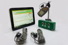
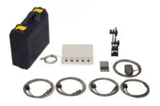
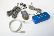
ಪ್ರಾಯೋಗಿಕವಾಗಿ, ಮುನ್ಸೂಚನೆಯ ಗುಣಮಾನವು ಅದನ್ನು ನೀಡುವ ಡೇಟಾದಷ್ಟೇ ಉತ್ತಮವಾಗಿದೆ, ಆದ್ದರಿಂದ ಮಾಪನ ಹೆಜ್ಜೆಯು ಗಣಿತವಷ್ಟೇ ಮುಖ್ಯವಾಗಿದೆ. ಪೋರ್ಟಬಲ್ ಎರಡು-ಚಾನೆಲ್ ಯಂತ್ರ ಸೇ ಬ್ಯಾಲೆನ್ಸೆಟ್-1ಎ ತಾಂತ್ರಿಕರನಿಗೆ ಪ್ರತಿ ಮಾರ್ಗ ಭೇಟಿದಲ್ಲಿ ಪುನರಾವರ್ತಿತವಲ್ಲದ ರೋಹಿತಗಳು ಮತ್ತು ಸಂಗ್ರಹವನ್ನು ಅನುಮತಿಸುತ್ತದೆ amplitude ಓದುವಿಕೆಗಳು ಯಾವುದೇ ಶೇಷ-ಜೀವನ ಅಂದಾಜು ನಿರ್ಮಿತವಾದ ಸಮಂಜಸ ಪ್ರವೃತ್ತಿ ಬಿಂದುಗಳಿಂದ. ಮುನ್ಸೂಚನೆಯು, ಅಂತಿಮವಾಗಿ, ನಿಜವಾದ ಪೂರ್ವಸೂಚಕ ನಿರ್ವಹಣೆಯನ್ನು ಸುಮಾರು ಪ್ರತ್ಯೇಕಿಸುವ ಅಂಶವಾಗಿದೆ ಸ್ಥಿತಿ ಮೇಲ್ವಿಚಾರಣೆ: ಪ್ರವೃತ್ತಿ ಡೇಟಾ ಮತ್ತು ದೋಷ ಪ್ರಗತಿಯ ತಿಳುವಳಿಕೆಯಿಂದ ವಿಫಲತೆಯ ಸಮಯಾವಧಿಯನ್ನು ಮುನ್ಸೂಚಿಸುವ ಮೂಲಕ, ಇದು ಯಂತ್ರೋಪಯೋಗಿತೆಯನ್ನು ಗರಿಷ್ಠ ಮಾಡುವಾಗ ವಿಶ್ವಾಸಾರ್ಹತೆಯನ್ನು ರಕ್ಷಿಸುವ ಸಂಪ್ರಕ್ಕವಿತವಾದ ಸಮಯವನ್ನು ಸಕ್ರಿಯ ಮಾಡುತ್ತದೆ.
