
PORTABLE BALANCER "BALANSET-1A"
A Dual-Channel PC-Based Dynamic Balancing System
OPERATION MANUAL
rev. 1.56 May 2023
2023 | Estonia, Narva
SAFETY NOTICE: This device complies with EU safety standards. Class 2 Laser Product. Follow rotating equipment safety procedures. See full safety information below →
1. BALANCING SYSTEM OVERVIEW
Balanset-1A balancer provides single- and two-plane dynamic balancing services for fans, grinding wheels, spindles, crushers, pumps and other rotating machinery.
Balanset-1A balancer includes two vibrosensors (accelerometers), laser phase sensor (tachometer), 2-channel USB interface unit with pre-amplifiers, integrators and ADC acquisition module and Windows based balancing software. Balanset-1A requires notebook or other Windows (WinXP...Win11, 32 or 64bit) compatible PC.
Balancing software provides the correct balancing solution for single-plane and two-plane balancing automatically. ಬ್ಯಾಲೆನ್ಸೆಟ್-1ಎ is simple to use for non-vibration experts.
All balancing results saved in archive and can be used to create the reports.
ಮುಖ್ಯ ಲಕ್ಷಣಗಳು
Easy to Use
- • User selectable trial mass
- • Trial mass validity popup
- • Manual data input
Measurement Capabilities
- • RPM, amplitude and phase
- • FFT spectrum analysis
- • Waveform and spectrum display
- • Dual-channel simultaneous data
Advanced Functions
- • Saved influence coefficients
- • Trim balancing
- • Mandrel eccentricity calc.
- • ISO 1940 tolerance calc.
ದತ್ತಾಂಶ ನಿರ್ವಹಣೆ
- • Unlimited balancing data storage
- • Vibration waveform storage
- • Archive and reports
Calculation Tools
- • Split weight calculation
- • Drill calculation
- • Changing correction planes
- • Polar graph visualization
Analysis Options
- • Remove or leave trial weights
- • RunDown charts (experimental)
2. SPECIFICATION
| ಪ್ಯಾರಾಮೀಟರ್ | Specification |
|---|---|
| Measurement range of the root-mean-square value (RMS) of the vibration velocity, mm/sec (for 1x vibration) | from 0.2 to 80 |
| The frequency range of the RMS measurement of the vibration velocity, Hz | from 5 to 1000 (amplitude error ≤10% above 550 Hz) |
| Number of the correction planes | 1 or 2 |
| Range of the frequency of rotation measurement, rpm | 250 – 90000 |
| Range of the vibration phase measurement, angular degrees | from 0 to 360 |
| Error of the vibration phase measurement, angular degrees | ± 1 |
| Measurement accuracy of RMS vibration velocity | ±(0.1 + 0.1×Vಅಳೆಯಲಾದ) mm/sec |
| Measurement accuracy of rotation frequency | ±(1 + 0.005×Nಅಳೆಯಲಾದ) rpm |
| Mean time between failures (MTBF), hours, min | 1000 |
| Average service life, years, min | 6 |
| Dimensions (in hard case), cm | 39*33*13 |
| Mass, kg | <5 |
| Overall dimensions of the vibrator sensor, mm, max | 25*25*20 |
| Mass of the vibrator sensor, kg, max | 0.04 |
|
ಕಾರ್ಯಾಚರಣಾ ಪರಿಸ್ಥಿತಿಗಳು: - Temperature range: from 5°C to 50°C - Relative humidity: < 85%, unsaturated - Without strong electric-magnetic field & strong impact |
|
3. PACKAGE
Balanset-1A balancer includes two single-axis accelerometers, laser phase reference marker (digital tachometer), 2-channel USB interface unit with pre-amplifiers, integrators and ADC acquisition module and Windows based balancing software.
Delivery Set
| Description | Number | Note |
|---|---|---|
| USB interface unit | 1 | |
| Laser phase reference marker (tachometer) | 1 | |
| Single-axis accelerometers | 2 | |
| Magnetic stand | 1 | |
| Digital scales | 1 | |
| Hard case for transportation | 1 | |
| "Balanset-1A". User's manual. | 1 | |
| Flash disk with balancing software | 1 |
4. BALANCE PRINCIPLES
4.1. "Balanset-1A" includes (fig. 4.1) USB interface unit (1), two accelerometers (2) and (3), phase reference marker (4) and portable PC (not supplied) (5).
Delivery set also includes the magnetic stand (6) ) used for mounting the phase reference marker and digital scales 7.
X1 and X2 connectors intended for connection of the vibration sensors respectively to 1 and 2 measuring channels, and the X3 connector used for connection of the phase reference marker.
The USB cable provides power supply and connection of the USB interface unit to the computer.

Fig. 4.1. Delivery set of the "Balanset-1A"
Mechanical vibrations cause an electrical signal proportional to the vibration acceleration on the output of the vibration sensor. Digitized signals from ADC module transferred via USB to the portable PC ( (5). Phase reference marker generates the pulse signal used to calculate rotation frequency and vibration phase angle. Windows based software provides solution for single-plane and two-plane balancing, spectrum analyzing, charts, reports, storage of influence coefficients
5. SAFETY PRECAUTIONS
⚡ ATTENTION - Electrical Safety
5.1. When operating on 220V electrical safety regulations must be observed. It is not allowed to repair the device when connected to 220 V.
5.2. If you use the appliance in a low quality AC power environment or in the presence of network interference it is recommended to use standalone power from computer's battery pack.
⚠️ Additional Safety Requirements for Rotating Equipment
- !Machine Lockout: Always implement proper lockout/tagout procedures before installing sensors
- !Personal Protective Equipment: Wear safety glasses, hearing protection, and avoid loose clothing near rotating machinery
- !Secure Installation: Ensure all sensors and cables are securely fastened and cannot be caught by rotating parts
- !Emergency Procedures: Know location of emergency stops and shutdown procedures
- !Training: Only trained personnel should operate balancing equipment on rotating machinery
6. SOFTWARE AND HARDWARE SETTINGS
6.1. USB drivers and balancing software installation
Before working install drivers and balancing software.
List of folders and files
Installation disk (flash drive) contains the following files and folders:
- Bs1Av###Setup – folder with "Balanset-1A" balancing software (### – version number)
- ArdDrv – USB drivers
- EBalancer_manual.pdf – this manual
- Bal1Av###Setup.exe – setup file. This file contains all archived files and folders mentioned above. ### – version of "Balanset-1A" software.
- Ebalanc.cfg – sensitivity value
- Bal.ini – some initialization data
Software Installation procedure
For installing drivers and specialized software run file Bal1Av###Setup.exe and follow setup instructions by pressing buttons «Next», «ОК» etc.
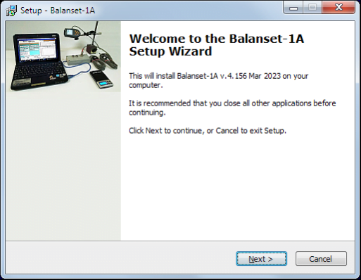
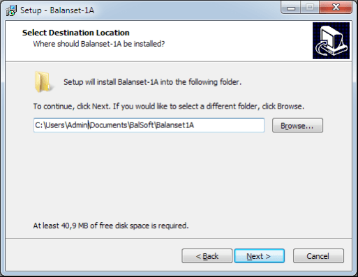
Choose setup folder. Usually the given folder should not be changed.
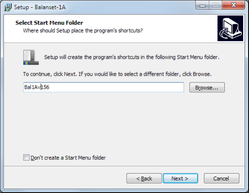
Then the program requires specifying Program group and desktop folders. Press button Next.
Finishing Installation
- ✓Install sensors on the inspected or balanced mechanism (Detailed information about how to install the sensors is given in Annex 1)
- ✓Connect vibration sensors 2 and 3 to the inputs X1 and X2, and phase angle sensor to the input X3 of USB interface unit.
- ✓Connect USB interface unit to the USB-port of the computer.
- ✓When using the AC power supply connect the computer to the power mains. Connect the power supply to 220 V, 50 Hz.
- ✓Click shortcut "Balanset-1A" on desktop.
7. BALANCING SOFTWARE
7.1. General
Initial window
When running the program "Balanset-1A" the Initial window, shown in Fig. 7.1, appears.

Fig. 7.1. Initial window of the "Balanset-1A"
There are 9 buttons in the Initial window with the names of the functions realized when click on them.
F1-«About»
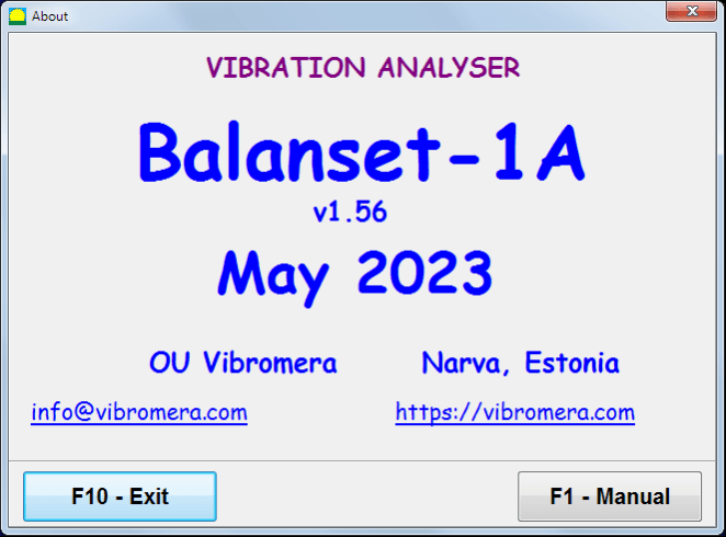
Fig. 7.2. F1-«About» window
F2-«Single plane», F3-«Two plane»
Pressing "F2- ಏಕ-ಸಮತಲ" (or F2 function key on the computer keyboard) selects the measurement vibration on the X1.
After clicking this button, the computer display diagram shown in Fig. 7.1 illustrating a process of measuring the vibration only on the first measuring channel (or the balancing process in a single plane).
Pressing the "F3-ಎರಡು-ಪ್ಲೇನ್" (or F3 function key on the computer keyboard) selects the mode of vibration measurements on two channels X1 and X2 simultaneously. (Fig. 7.3.)
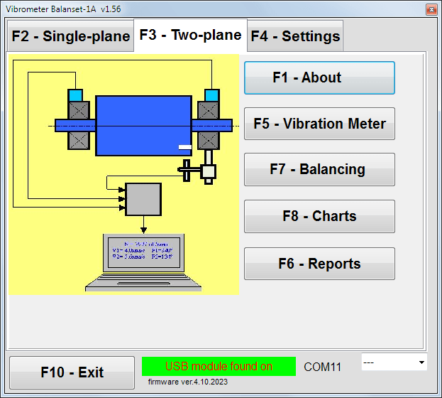
Fig. 7.3. Initial window of the "Balanset-1A". Two plane balancing.
F4 – «Settings»
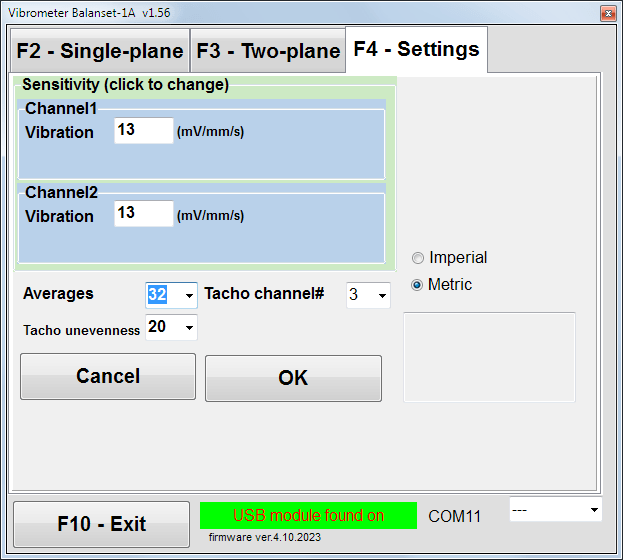
Fig. 7.4. "Settings" window
In this window you can change some Balanset-1A settings.
- Sensitivity. The nominal value is 13 mV / mm/s.
Changing the sensitivity coefficients of sensors is required only when replacing sensors!
ಗಮನ!
When you enter a sensitivity coefficient its fractional part is separated from the integer part with the decimal point (the sign ",").
- Averaging – number of averaging (number of revolutions of the rotor over which data is averaged to more accuracy)
- Tacho channel# - channel# the Tacho is connected. By default - 3rd channel.
- Unevenness - the difference in duration between adjacent tacho pulses, which above gives the warning "Failure of the tachometer"
- Imperial/Metric - Select the system of units.
Com port number is assigned automatically.
F5 – «Vibration meter»
Pressing this button (or a function key of F5 on the computer keyboard) activates the mode of vibration measurement on one or two measuring channels of virtual Vibration meter depending on the buttons condition “F2-single-plane", "F3-two-plane".
F6 – «Reports»
Pressing this button (or F6 function key on the computer keyboard) switches on the balancing Archive, from which you can print the report with the results of balancing for a specific mechanism (rotor).
F7 – «Balancing»
Pressing this button (or function key F7 on your keyboard) activates balancing mode in one or two correction planes depending on which measurement mode is selected by pressing the buttons “F2-single-plane", "F3-two-plane".
F8 – «Charts»
Pressing this button (or F8 function key on the computer’s keyboard) enables graphic Vibration meter, the implementation of which displays on a display simultaneously with the digital values of the amplitude and phase of the vibration graphics of its time function.
F10 – «Exit»
Pressing this button (or F10 function key on the computer's keyboard) completes the program "Balanset-1A".
7.2. "Vibration meter"
Before working in the "Vibration meter" mode, install vibration sensors on the machine and connect them respectively to the connectors X1 and X2 of the USB interface unit. Tacho sensor should be connected to the input X3 of the USB interface unit.

Fig. 7.5 USB interface unit
Place reflective tape on the surface of a rotor for tacho working.

Fig. 7.6. Reflective tape.
Recommendations for the installation and configuration of sensors are given in Annex 1.
To begin the measurement in the Vibration meter mode click on the button "F5 – Vibration Meter" in the Initial window of the program (see fig. 7.1).
Vibration Meter window appears (see. Fig.7.7)

Fig. 7.7. Vibration meter mode. Wave and Spectrum.
To start vibration measurements click button "F9 – Run" (or press the function key F9 on the keyboard).
If Trigger mode Auto is checked – the results of vibration measurements will be periodically displayed on the screen.
In case of simultaneous measurement of vibration on the first and second channels, the windows located beneath the words “Plane 1" and "Plane 2" will be filled.
Vibration measuring in the “Vibration” mode also may be carried out with disconnected phase angle sensor. In the Initial window of the program the value of the total RMS vibration (V1s, V2s) will only be displayed.
There are next settings in Vibration meter mode
- RMS Low, Hz – lowest frequency to calculate RMS of overall vibration
- ಬ್ಯಾಂಡ್ವಿಡ್ತ್ - vibration frequency bandwidth in the chart
- Averages - number of average for more measure accuracy
To complete the work in the "Vibration meter" mode click button "F10 – Exit" and return to the Initial window.

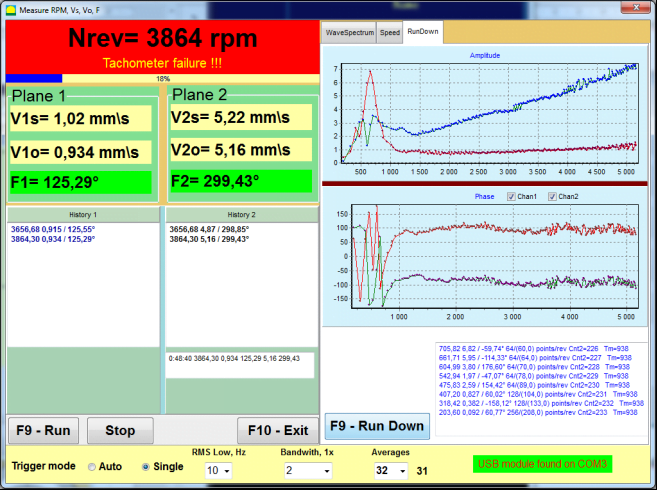
Fig. 7.8. Vibration meter mode. Rotation speed Unevenness, 1x vibration wave form.
Fig. 7.9. Vibration meter mode. Rundown (beta version, no warranty!).
7.3 Balancing procedure
ಉತ್ತಮ ತಾಂತ್ರಿಕ ಸ್ಥಿತಿಯಲ್ಲಿ ಮತ್ತು ಸರಿಯಾಗಿ ಜೋಡಿಸಲಾದ ಕಾರ್ಯವಿಧಾನಗಳಿಗೆ ಸಮತೋಲನವನ್ನು ನಡೆಸಲಾಗುತ್ತದೆ. ಇಲ್ಲದಿದ್ದರೆ, ಸಮತೋಲನಗೊಳಿಸುವ ಮೊದಲು ಯಾಂತ್ರಿಕ ವ್ಯವಸ್ಥೆಯನ್ನು ಸರಿಪಡಿಸಬೇಕು, ಸರಿಯಾದ ಬೇರಿಂಗ್ಗಳಲ್ಲಿ ಸ್ಥಾಪಿಸಬೇಕು ಮತ್ತು ಸರಿಪಡಿಸಬೇಕು. ರೋಟರ್ ಅನ್ನು ಕಲ್ಮಶಗಳಿಂದ ಸ್ವಚ್ಛಗೊಳಿಸಬೇಕು, ಅದು ಸಮತೋಲನ ಪ್ರಕ್ರಿಯೆಗೆ ಅಡ್ಡಿಯಾಗಬಹುದು.
ಮುಖ್ಯವಾಗಿ ಕಂಪನವು 1x ಕಂಪನವಾಗಿದೆ ಎಂದು ಖಚಿತಪಡಿಸಿಕೊಳ್ಳಲು ಕಂಪನ ಮೀಟರ್ ಮೋಡ್ನಲ್ಲಿ (F5 ಬಟನ್) ಕಂಪನವನ್ನು ಸಮತೋಲನಗೊಳಿಸುವ ಮೊದಲು.
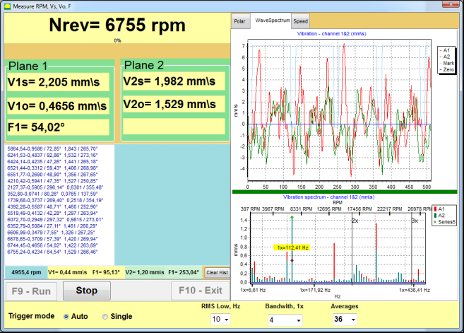
ಚಿತ್ರ 7.10. ಕಂಪನ ಮೀಟರ್ ಮೋಡ್. ಒಟ್ಟಾರೆ (V1s,V2s) ಮತ್ತು 1x (V1o,V2o) ಕಂಪನವನ್ನು ಪರಿಶೀಲಿಸಲಾಗುತ್ತಿದೆ.
If the value of the overall vibration V1s (V2s) is approximately equal to the magnitude of the vibration at rotational frequency (1x vibration) V1o (V2o), it can be assumed that the main contribution to the vibration mechanism comes from an imbalance of the rotor. If the value of the overall vibration V1s (V2s) is much higher than the 1x vibration component V1o (V2o), it is recommended to check the condition of the mechanism – condition of bearings, its mount on the base, ensure no contact between the fixed parts and the rotor during rotation, etc.
ಕಂಪನ ಮೀಟರ್ ಮೋಡ್ನಲ್ಲಿ ಅಳತೆ ಮಾಡಲಾದ ಮೌಲ್ಯಗಳ ಸ್ಥಿರತೆಗೆ ಸಹ ನೀವು ಗಮನ ಕೊಡಬೇಕು - ಕಂಪನದ ವೈಶಾಲ್ಯ ಮತ್ತು ಹಂತವು ಮಾಪನ ಪ್ರಕ್ರಿಯೆಯಲ್ಲಿ 10-15% ಗಿಂತ ಹೆಚ್ಚು ಬದಲಾಗಬಾರದು. ಇಲ್ಲದಿದ್ದರೆ, ಯಾಂತ್ರಿಕತೆಯು ಅನುರಣನ ಡೊಮೇನ್ಗೆ ಹತ್ತಿರದಲ್ಲಿ ಕಾರ್ಯನಿರ್ವಹಿಸುತ್ತಿದೆ ಎಂದು ಭಾವಿಸಬಹುದು. ಈ ಸಂದರ್ಭದಲ್ಲಿ, ರೋಟರ್ನ ತಿರುಗುವಿಕೆಯ ವೇಗವನ್ನು ಬದಲಾಯಿಸಿ, ಮತ್ತು ಇದು ಸಾಧ್ಯವಾಗದಿದ್ದರೆ - ಅಡಿಪಾಯದ ಮೇಲೆ ಯಂತ್ರದ ಅನುಸ್ಥಾಪನೆಯ ಪರಿಸ್ಥಿತಿಗಳನ್ನು ಬದಲಾಯಿಸಿ (ಉದಾಹರಣೆಗೆ, ಸ್ಪ್ರಿಂಗ್ ಬೆಂಬಲಗಳಲ್ಲಿ ತಾತ್ಕಾಲಿಕವಾಗಿ ಹೊಂದಿಸುವುದು).
For rotor balancing the ಪ್ರಭಾವ ಗುಣಾಂಕ ವಿಧಾನ of balancing (3-run method) should be used.
ಕಂಪನ ಬದಲಾವಣೆ, ದ್ರವ್ಯರಾಶಿ ಮತ್ತು ತಿದ್ದುಪಡಿ ತೂಕದ ಅನುಸ್ಥಾಪನೆಯ ಸ್ಥಳ (ಕೋನ) ಮೇಲೆ ಪ್ರಯೋಗ ದ್ರವ್ಯರಾಶಿಯ ಪರಿಣಾಮವನ್ನು ನಿರ್ಧರಿಸಲು ಪ್ರಾಯೋಗಿಕ ರನ್ಗಳನ್ನು ಮಾಡಲಾಗುತ್ತದೆ.
ಮೊದಲು ಯಾಂತ್ರಿಕತೆಯ ಮೂಲ ಕಂಪನವನ್ನು ನಿರ್ಧರಿಸಿ (ತೂಕವಿಲ್ಲದೆ ಮೊದಲ ಪ್ರಾರಂಭ), ತದನಂತರ ಪ್ರಾಯೋಗಿಕ ತೂಕವನ್ನು ಮೊದಲ ಸಮತಲಕ್ಕೆ ಹೊಂದಿಸಿ ಮತ್ತು ಎರಡನೇ ಪ್ರಾರಂಭವನ್ನು ಮಾಡಿದೆ. ನಂತರ, ಮೊದಲ ಸಮತಲದಿಂದ ಪ್ರಾಯೋಗಿಕ ತೂಕವನ್ನು ತೆಗೆದುಹಾಕಿ, ಎರಡನೇ ಸಮತಲದಲ್ಲಿ ಹೊಂದಿಸಿ ಮತ್ತು ಎರಡನೇ ಪ್ರಾರಂಭವನ್ನು ಮಾಡಿದರು.
ನಂತರ ಪ್ರೋಗ್ರಾಂ ಲೆಕ್ಕಾಚಾರ ಮತ್ತು ತಿದ್ದುಪಡಿ ತೂಕದ ಅನುಸ್ಥಾಪನೆಯ ತೂಕ ಮತ್ತು ಸ್ಥಳ (ಕೋನ) ಪರದೆಯ ಮೇಲೆ ಸೂಚಿಸುತ್ತದೆ.
ಒಂದೇ ಸಮತಲದಲ್ಲಿ ಸಮತೋಲನ ಮಾಡುವಾಗ (ಸ್ಥಿರ), ಎರಡನೇ ಪ್ರಾರಂಭವು ಅಗತ್ಯವಿಲ್ಲ.
ಪ್ರಾಯೋಗಿಕ ತೂಕವನ್ನು ರೋಟರ್ನಲ್ಲಿ ಅನಿಯಂತ್ರಿತ ಸ್ಥಳಕ್ಕೆ ಹೊಂದಿಸಲಾಗಿದೆ, ಅಲ್ಲಿ ಅದು ಅನುಕೂಲಕರವಾಗಿರುತ್ತದೆ, ಮತ್ತು ನಂತರ ನಿಜವಾದ ತ್ರಿಜ್ಯವನ್ನು ಸೆಟಪ್ ಪ್ರೋಗ್ರಾಂನಲ್ಲಿ ನಮೂದಿಸಲಾಗುತ್ತದೆ.
(ಸ್ಥಾನದ ತ್ರಿಜ್ಯವನ್ನು ಗ್ರಾಂ * ಎಂಎಂನಲ್ಲಿ ಅಸಮತೋಲನದ ಮೊತ್ತವನ್ನು ಲೆಕ್ಕಾಚಾರ ಮಾಡಲು ಮಾತ್ರ ಬಳಸಲಾಗುತ್ತದೆ)
ಪ್ರಮುಖ!
- ಯಾಂತ್ರಿಕತೆಯ ತಿರುಗುವಿಕೆಯ ನಿರಂತರ ವೇಗದೊಂದಿಗೆ ಅಳತೆಗಳನ್ನು ಕೈಗೊಳ್ಳಬೇಕು!
- ಪ್ರಯೋಗ ತೂಕದ ಅದೇ ತ್ರಿಜ್ಯದಲ್ಲಿ ತಿದ್ದುಪಡಿ ತೂಕವನ್ನು ಸ್ಥಾಪಿಸಬೇಕು!
ಪ್ರಾಯೋಗಿಕ ತೂಕದ ದ್ರವ್ಯರಾಶಿಯನ್ನು ಆಯ್ಕೆಮಾಡಲಾಗುತ್ತದೆ ಆದ್ದರಿಂದ ಅದರ ಅನುಸ್ಥಾಪನೆಯ ನಂತರ (> 20-30 °) ಮತ್ತು (20-30%) ಕಂಪನದ ವೈಶಾಲ್ಯವು ಗಮನಾರ್ಹವಾಗಿ ಬದಲಾಗುತ್ತದೆ. ಬದಲಾವಣೆಗಳು ತುಂಬಾ ಚಿಕ್ಕದಾಗಿದ್ದರೆ, ನಂತರದ ಲೆಕ್ಕಾಚಾರಗಳಲ್ಲಿ ದೋಷವು ಹೆಚ್ಚು ಹೆಚ್ಚಾಗುತ್ತದೆ. ಹಂತದ ಗುರುತು ಇರುವ ಅದೇ ಸ್ಥಳದಲ್ಲಿ (ಅದೇ ಕೋನ) ಪ್ರಾಯೋಗಿಕ ದ್ರವ್ಯರಾಶಿಯನ್ನು ಅನುಕೂಲಕರವಾಗಿ ಹೊಂದಿಸಿ.
Trial Weight Mass Calculation Formula
Mt = Mr × Ksupport × Kvibration / (Rt × (N/100)²)
ಎಲ್ಲಿ:
- Mt - trial weight mass, g
- Mr - rotor mass, g
- Ksupport - support stiffness coefficient (1-5)
- Kvibration - vibration level coefficient (0.5-2.5)
- Rt - trial weight installation radius, cm
- N - rotor speed, rpm
Support stiffness coefficient (Ksupport):
- 1.0 - Very soft supports (rubber dampers)
- 2.0-3.0 - Medium stiffness (standard bearings)
- 4.0-5.0 - Rigid supports (massive foundation)
Vibration level coefficient (Kvibration):
- 0.5 - Low vibration (up to 5 mm/sec)
- 1.0 - Normal vibration (5-10 mm/sec)
- 1.5 - Elevated vibration (10-20 mm/sec)
- 2.0 - High vibration (20-40 mm/sec)
- 2.5 - Very high vibration (>40 mm/sec)
🔗 Use our online calculator:
Trial Weight Calculator →⚠️ Important!
ಪ್ರತಿ ಪರೀಕ್ಷೆಯ ನಂತರ ಪ್ರಯೋಗ ಸಮೂಹವನ್ನು ತೆಗೆದುಹಾಕಲಾಗುತ್ತದೆ! ಪ್ರಯೋಗ ತೂಕದ ಅನುಸ್ಥಾಪನೆಯ ಸ್ಥಳದಿಂದ ಲೆಕ್ಕ ಹಾಕಿದ ಕೋನದಲ್ಲಿ ಹೊಂದಿಸಲಾದ ತಿದ್ದುಪಡಿ ತೂಕ ರೋಟರ್ ತಿರುಗುವ ದಿಕ್ಕಿನಲ್ಲಿ!
Angle Calculation Explanation:
The correction weight installation angle is ALWAYS counted from the trial weight installation point in the direction of rotor rotation.
- Zero Point (0°): The exact location where you installed the trial weight becomes your reference point (0 degrees).
- ದಿಕ್ಕು: Measure the angle in the same direction the rotor spins.
Example: If the rotor spins clockwise, measure the angle clockwise from the trial weight position. - ವ್ಯಾಖ್ಯಾನ: If the program displays an angle of 120°, you must install the correction weight 120 degrees ahead of the trial weight position in the direction of rotation.
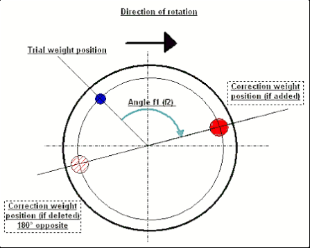
Fig. 7.11. Correction weight mounting.
Recommended!
ಡೈನಾಮಿಕ್ ಬ್ಯಾಲೆನ್ಸಿಂಗ್ ಮಾಡುವ ಮೊದಲು, ಸ್ಥಿರ ಅಸಮತೋಲನವು ತುಂಬಾ ಹೆಚ್ಚಿಲ್ಲ ಎಂದು ಖಚಿತಪಡಿಸಿಕೊಳ್ಳಲು ಸೂಚಿಸಲಾಗುತ್ತದೆ. ಸಮತಲ ಅಕ್ಷದೊಂದಿಗೆ ರೋಟರ್ಗಳಿಗೆ, ರೋಟರ್ ಅನ್ನು ಪ್ರಸ್ತುತ ಸ್ಥಾನದಿಂದ 90 ಡಿಗ್ರಿ ಕೋನದಿಂದ ಹಸ್ತಚಾಲಿತವಾಗಿ ತಿರುಗಿಸಬಹುದು. ರೋಟರ್ ಸ್ಥಿರವಾಗಿ ಅಸಮತೋಲಿತವಾಗಿದ್ದರೆ, ಅದನ್ನು ಸಮತೋಲನದ ಸ್ಥಾನಕ್ಕೆ ತಿರುಗಿಸಲಾಗುತ್ತದೆ. ರೋಟರ್ ಸಮತೋಲನದ ಸ್ಥಾನವನ್ನು ಪಡೆದ ನಂತರ, ರೋಟರ್ ಉದ್ದದ ಮಧ್ಯ ಭಾಗದಲ್ಲಿ ಮೇಲಿನ ಹಂತದಲ್ಲಿ ತೂಕದ ಸಮತೋಲನವನ್ನು ಹೊಂದಿಸುವುದು ಅವಶ್ಯಕ. ರೋಟರ್ ಯಾವುದೇ ಸ್ಥಾನದಲ್ಲಿ ಚಲಿಸದ ರೀತಿಯಲ್ಲಿ ತೂಕದ ತೂಕವನ್ನು ಆಯ್ಕೆ ಮಾಡಬೇಕು.
ಅಂತಹ ಪೂರ್ವ-ಸಮತೋಲನವು ಬಲವಾಗಿ ಅಸಮತೋಲಿತ ರೋಟರ್ನ ಮೊದಲ ಪ್ರಾರಂಭದಲ್ಲಿ ಕಂಪನದ ಪ್ರಮಾಣವನ್ನು ಕಡಿಮೆ ಮಾಡುತ್ತದೆ.
Sensor installation and mounting
ವಿಆಯ್ದ ಅಳತೆ ಬಿಂದುವಿನಲ್ಲಿ ಯಂತ್ರದಲ್ಲಿ ibration ಸಂವೇದಕವನ್ನು ಸ್ಥಾಪಿಸಬೇಕು ಮತ್ತು USB ಇಂಟರ್ಫೇಸ್ ಘಟಕದ ಇನ್ಪುಟ್ X1 ಗೆ ಸಂಪರ್ಕಿಸಬೇಕು.
There are two mounting configurations:
- Magnets
- ಥ್ರೆಡ್ ಸ್ಟಡ್ M4
ಆಪ್ಟಿಕಲ್ ಟ್ಯಾಕೋ ಸಂವೇದಕವನ್ನು USB ಇಂಟರ್ಫೇಸ್ ಘಟಕದ ಇನ್ಪುಟ್ X3 ಗೆ ಸಂಪರ್ಕಿಸಬೇಕು. ಇದಲ್ಲದೆ, ಈ ಸಂವೇದಕವನ್ನು ಬಳಸಲು ರೋಟರ್ನ ಮೇಲ್ಮೈಯಲ್ಲಿ ವಿಶೇಷ ಪ್ರತಿಫಲಿತ ಗುರುತು ಅನ್ವಯಿಸಬೇಕು.
📏 Optical Sensor Installation Requirements
- ✓Distance to rotor surface: 50-500 mm (depending on sensor model)
- ✓Reflective tape width: Minimum 1-1.5 cm (depends on speed and radius)
- ✓Orientation: Perpendicular to rotor surface
- ✓ಅಳವಡಿಕೆ: Use magnetic stand or clamp for stable positioning
- ✓Avoid direct sunlight or bright artificial lighting on sensor/tape
💡 Tape width calculation: For optimal performance, calculate tape width using:
L ≥ (N × R)/30000 ≥ 1.0-1.5 cm
Where: L - tape width (cm), N - rotor speed (rpm), R - tape radius (cm)
ಸಂವೇದಕಗಳ ಸೈಟ್ ಆಯ್ಕೆಯ ವಿವರವಾದ ಅವಶ್ಯಕತೆಗಳು ಮತ್ತು ಸಮತೋಲನ ಮಾಡುವಾಗ ವಸ್ತುವಿಗೆ ಅವುಗಳ ಲಗತ್ತನ್ನು ಅನೆಕ್ಸ್ 1 ರಲ್ಲಿ ಹೊಂದಿಸಲಾಗಿದೆ.
7.4 Single plane balancing
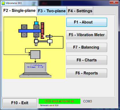
Fig. 7.12. "Single plane balancing"
Balancing Archive
To start working on the program in the "ಏಕ-ಪ್ಲೇನ್ ಸಮತೋಲನ" mode, click on the "F2-ಏಕ-ವಿಮಾನ" button (or press the F2 key on the computer keyboard).
Then click on the "F7 - ಸಮತೋಲನ" button, after which the ಸಿಂಗಲ್ ಪ್ಲೇನ್ ಬ್ಯಾಲೆನ್ಸಿಂಗ್ ಆರ್ಕೈವ್ ವಿಂಡೋ ಕಾಣಿಸಿಕೊಳ್ಳುತ್ತದೆ, ಇದರಲ್ಲಿ ಸಮತೋಲನ ಡೇಟಾವನ್ನು ಉಳಿಸಲಾಗುತ್ತದೆ (Fig. 7.13 ನೋಡಿ).

ಚಿತ್ರ 7.13 ಏಕ ಸಮತಲದಲ್ಲಿ ಬ್ಯಾಲೆನ್ಸಿಂಗ್ ಆರ್ಕೈವ್ ಅನ್ನು ಆಯ್ಕೆ ಮಾಡುವ ವಿಂಡೋ.
ಈ ವಿಂಡೋದಲ್ಲಿ, ನೀವು ರೋಟರ್ ಹೆಸರಿನಲ್ಲಿ ಡೇಟಾವನ್ನು ನಮೂದಿಸಬೇಕಾಗಿದೆ (ರೋಟರ್ ಹೆಸರು), ರೋಟರ್ ಸ್ಥಾಪನೆಯ ಸ್ಥಳ (ಸ್ಥಳ), ಕಂಪನ ಮತ್ತು ಉಳಿದ ಅಸಮತೋಲನಕ್ಕೆ ಸಹಿಷ್ಣುತೆಗಳು (ಸಹಿಷ್ಣುತೆ), ಅಳತೆಯ ದಿನಾಂಕ. ಈ ಡೇಟಾವನ್ನು ಡೇಟಾಬೇಸ್ನಲ್ಲಿ ಸಂಗ್ರಹಿಸಲಾಗಿದೆ. ಅಲ್ಲದೆ, Arc### ಫೋಲ್ಡರ್ ಅನ್ನು ರಚಿಸಲಾಗಿದೆ, ಅಲ್ಲಿ ### ಎಂಬುದು ಚಾರ್ಟ್ಗಳು, ವರದಿ ಫೈಲ್ ಇತ್ಯಾದಿಗಳನ್ನು ಉಳಿಸುವ ಆರ್ಕೈವ್ನ ಸಂಖ್ಯೆ. ಬ್ಯಾಲೆನ್ಸಿಂಗ್ ಪೂರ್ಣಗೊಂಡ ನಂತರ, ಬಿಲ್ಟ್-ಇನ್ ಎಡಿಟರ್ನಲ್ಲಿ ಸಂಪಾದಿಸಬಹುದಾದ ಮತ್ತು ಮುದ್ರಿಸಬಹುದಾದ ವರದಿಯ ಫೈಲ್ ಅನ್ನು ರಚಿಸಲಾಗುತ್ತದೆ.
ಅಗತ್ಯ ಡೇಟಾವನ್ನು ನಮೂದಿಸಿದ ನಂತರ, ನೀವು ಕ್ಲಿಕ್ ಮಾಡಬೇಕಾಗುತ್ತದೆ "F10-OK" button, after which the "ಏಕ-ಪ್ಲೇನ್ ಸಮತೋಲನ" window will open (see Fig. 7.13)
ಬ್ಯಾಲೆನ್ಸಿಂಗ್ ಸೆಟ್ಟಿಂಗ್ಗಳು (1-ಪ್ಲೇನ್)
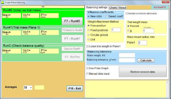
ಚಿತ್ರ 7.14. ಏಕ ವಿಮಾನ. ಸಮತೋಲನ ಸೆಟ್ಟಿಂಗ್ಗಳು
In the left side of this window displays the data of vibration measurements and the measurement control buttons "Run # 0", "# 1 ರನ್ ಮಾಡಿ", "ರನ್ಟ್ರಿಮ್".
ಈ ವಿಂಡೋದ ಬಲಭಾಗದಲ್ಲಿ ಮೂರು ಟ್ಯಾಬ್ಗಳಿವೆ
- Balancing settings
- ಪಟ್ಟಿಯಲ್ಲಿ
- Result
The "Balancing settings" tab is used to enter the balancing settings:
- "Influence coefficient" -
- "ಹೊಸ ರೋಟರ್” - ಹೊಸ ರೋಟರ್ನ ಸಮತೋಲನದ ಆಯ್ಕೆ, ಇದಕ್ಕಾಗಿ ಯಾವುದೇ ಸಂಗ್ರಹಿಸಲಾದ ಸಮತೋಲನ ಗುಣಾಂಕಗಳಿಲ್ಲ ಮತ್ತು ತಿದ್ದುಪಡಿ ತೂಕದ ದ್ರವ್ಯರಾಶಿ ಮತ್ತು ಅನುಸ್ಥಾಪನಾ ಕೋನವನ್ನು ನಿರ್ಧರಿಸಲು ಎರಡು ರನ್ಗಳು ಅಗತ್ಯವಿದೆ.
- "Saved coeff.” – ರೋಟರ್ ಮರು-ಸಮತೋಲನದ ಆಯ್ಕೆ, ಇದಕ್ಕಾಗಿ ಉಳಿಸಿದ ಸಮತೋಲನ ಗುಣಾಂಕಗಳಿವೆ ಮತ್ತು ಸರಿಪಡಿಸುವ ತೂಕದ ತೂಕ ಮತ್ತು ಅನುಸ್ಥಾಪನಾ ಕೋನವನ್ನು ನಿರ್ಧರಿಸಲು ಕೇವಲ ಒಂದು ರನ್ ಅಗತ್ಯವಿದೆ.
- "Trial weight mass" -
- "Percent" - corrective weight is calculated as a percentage of the trial weight.
- "Gram" - the known mass of the trial weight is entered and the mass of the corrective weight is calculated in grams ಅಥವಾ ಒಳಗೆ oz ಸಾಮ್ರಾಜ್ಯಶಾಹಿ ವ್ಯವಸ್ಥೆಗಾಗಿ.
⚠️ Attention! If it is necessary to use the "Saved coeff.”ಆರಂಭಿಕ ಸಮತೋಲನದ ಸಮಯದಲ್ಲಿ ಹೆಚ್ಚಿನ ಕೆಲಸಕ್ಕಾಗಿ ಮೋಡ್, ಪ್ರಾಯೋಗಿಕ ತೂಕದ ದ್ರವ್ಯರಾಶಿಯನ್ನು ಗ್ರಾಂ ಅಥವಾ oz ನಲ್ಲಿ ನಮೂದಿಸಬೇಕು, % ನಲ್ಲಿ ಅಲ್ಲ. ವಿತರಣಾ ಪ್ಯಾಕೇಜ್ನಲ್ಲಿ ಮಾಪಕಗಳನ್ನು ಸೇರಿಸಲಾಗಿದೆ.
- "Weight Attachment Method"
- "Free position" - weights can be installed in an arbitrary angular positions on the circumference of the rotor.
- "Fixed position” – weight can be installed in fixed angular positions on the rotor, for example, on blades or holes (for example 12 holes – 30 degrees), etc. The number of fixed positions must be entered in the appropriate field. After balancing, the program will automatically split the weight into two parts and indicate the number of positions on which it is necessary to establish the masses obtained.
- "Circular groove" – used for grinding wheel balancing In this case 3 counterweights are used to eliminate unbalance
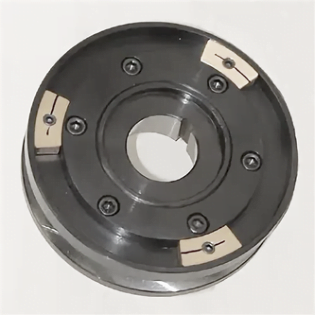
ಚಿತ್ರ 7.17 3 ಕೌಂಟರ್ವೈಟ್ಗಳೊಂದಿಗೆ ಗ್ರೈಂಡಿಂಗ್ ವೀಲ್ ಬ್ಯಾಲೆನ್ಸಿಂಗ್
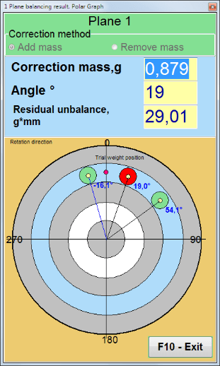
ಚಿತ್ರ 7.18 ಗ್ರೈಂಡಿಂಗ್ ವೀಲ್ ಬ್ಯಾಲೆನ್ಸಿಂಗ್. ಪೋಲಾರ್ ಗ್ರಾಫ್.

ಚಿತ್ರ 7.15. ಫಲಿತಾಂಶ ಟ್ಯಾಬ್. ತಿದ್ದುಪಡಿ ತೂಕದ ಆರೋಹಣದ ಸ್ಥಿರ ಸ್ಥಾನ.
Z1 and Z2 – positions of corrective weights installed, calculated from Z1 position according to rotation direction. Z1 is the position where the trial weight was installed.
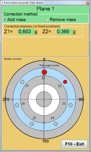
ಚಿತ್ರ 7.16 ಸ್ಥಿರ ಸ್ಥಾನಗಳು. ಧ್ರುವ ರೇಖಾಚಿತ್ರ.
- "Mass mount radius, mm" - "Plane1" - The radius of the trial weight in the 1 plane. It is required to calculate the magnitude of the initial and residual imbalance to determine compliance with the tolerance for residual imbalance after balancing.
- "ಪ್ಲೇನ್ 1 ರಲ್ಲಿ ಪ್ರಾಯೋಗಿಕ ತೂಕವನ್ನು ಬಿಡಿ.” ಸಾಮಾನ್ಯವಾಗಿ ವಿಚಾರಣೆಯ ತೂಕವನ್ನು ಸಮತೋಲನ ಪ್ರಕ್ರಿಯೆಯಲ್ಲಿ ತೆಗೆದುಹಾಕಲಾಗುತ್ತದೆ. ಆದರೆ ಕೆಲವು ಸಂದರ್ಭಗಳಲ್ಲಿ ಅದನ್ನು ತೆಗೆದುಹಾಕಲು ಅಸಾಧ್ಯವಾಗಿದೆ, ನಂತರ ಲೆಕ್ಕಾಚಾರದಲ್ಲಿ ಪ್ರಾಯೋಗಿಕ ತೂಕದ ದ್ರವ್ಯರಾಶಿಯನ್ನು ಲೆಕ್ಕಹಾಕಲು ನೀವು ಇದರಲ್ಲಿ ಚೆಕ್ ಮಾರ್ಕ್ ಅನ್ನು ಹೊಂದಿಸಬೇಕಾಗುತ್ತದೆ.
- "Manual data input"- ಕಂಪನ ಮೌಲ್ಯ ಮತ್ತು ಹಂತವನ್ನು ವಿಂಡೋದ ಎಡಭಾಗದಲ್ಲಿರುವ ಸೂಕ್ತ ಕ್ಷೇತ್ರಗಳಲ್ಲಿ ಹಸ್ತಚಾಲಿತವಾಗಿ ನಮೂದಿಸಲು ಮತ್ತು "ಗೆ ಬದಲಾಯಿಸುವಾಗ ತಿದ್ದುಪಡಿ ತೂಕದ ದ್ರವ್ಯರಾಶಿ ಮತ್ತು ಅನುಸ್ಥಾಪನಾ ಕೋನವನ್ನು ಲೆಕ್ಕಾಚಾರ ಮಾಡಲು ಬಳಸಲಾಗುತ್ತದೆ.Results" tab
- Button "ಅಧಿವೇಶನ ಡೇಟಾವನ್ನು ಮರುಸ್ಥಾಪಿಸಿ". ಸಮತೋಲನದ ಸಮಯದಲ್ಲಿ, ಅಳತೆ ಮಾಡಿದ ಡೇಟಾವನ್ನು session1.ini ಫೈಲ್ನಲ್ಲಿ ಉಳಿಸಲಾಗುತ್ತದೆ. ಕಂಪ್ಯೂಟರ್ ಘನೀಕರಿಸುವಿಕೆ ಅಥವಾ ಇತರ ಕಾರಣಗಳಿಗಾಗಿ ಮಾಪನ ಪ್ರಕ್ರಿಯೆಯು ಅಡಚಣೆಯಾಗಿದ್ದರೆ, ಈ ಗುಂಡಿಯನ್ನು ಕ್ಲಿಕ್ ಮಾಡುವುದರ ಮೂಲಕ ನೀವು ಮಾಪನ ಡೇಟಾವನ್ನು ಮರುಸ್ಥಾಪಿಸಬಹುದು ಮತ್ತು ಅಡಚಣೆಯ ಕ್ಷಣದಿಂದ ಸಮತೋಲನವನ್ನು ಮುಂದುವರಿಸಬಹುದು.
- Mandrel eccentricity elimination (Index balancing) ಮ್ಯಾಂಡ್ರೆಲ್ (ಆರ್ಬರ್ ಬ್ಯಾಲೆನ್ಸಿಂಗ್) ನ ವಿಕೇಂದ್ರೀಯತೆಯ ಪ್ರಭಾವವನ್ನು ತೊಡೆದುಹಾಕಲು ಹೆಚ್ಚುವರಿ ಪ್ರಾರಂಭದೊಂದಿಗೆ ಸಮತೋಲನಗೊಳಿಸುವುದು. ಗೆ ಸಂಬಂಧಿಸಿದಂತೆ 0 ° ಮತ್ತು 180 ° ನಲ್ಲಿ ಪರ್ಯಾಯವಾಗಿ ರೋಟರ್ ಅನ್ನು ಆರೋಹಿಸಿ. ಎರಡೂ ಸ್ಥಾನಗಳಲ್ಲಿ ಅಸಮತೋಲನವನ್ನು ಅಳೆಯಿರಿ.
- Balancing tolerance ಜಿಎಕ್ಸ್ ಎಂಎಂ (ಜಿ-ವರ್ಗಗಳು) ನಲ್ಲಿ ಉಳಿದ ಅಸಮತೋಲನ ಸಹಿಷ್ಣುತೆಗಳನ್ನು ನಮೂದಿಸುವುದು ಅಥವಾ ಲೆಕ್ಕಾಚಾರ ಮಾಡುವುದು
- Use Polar Graph Use polar graph to display balancing results
1-ಪ್ಲೇನ್ ಬ್ಯಾಲೆನ್ಸಿಂಗ್. ಹೊಸ ರೋಟರ್
As noted above, "ಹೊಸ ರೋಟರ್" balancing requires two test runs and at least one trim run of the balancing machine.
Run#0 (ಆರಂಭಿಕ ಓಟ)
ಬ್ಯಾಲೆನ್ಸಿಂಗ್ ರೋಟರ್ನಲ್ಲಿ ಸಂವೇದಕಗಳನ್ನು ಸ್ಥಾಪಿಸಿದ ನಂತರ ಮತ್ತು ಸೆಟ್ಟಿಂಗ್ಗಳ ನಿಯತಾಂಕಗಳನ್ನು ನಮೂದಿಸಿದ ನಂತರ, ರೋಟರ್ ತಿರುಗುವಿಕೆಯನ್ನು ಆನ್ ಮಾಡುವುದು ಅವಶ್ಯಕ ಮತ್ತು ಅದು ಕೆಲಸದ ವೇಗವನ್ನು ತಲುಪಿದಾಗ, ಒತ್ತಿರಿ "Run#0" button to start measurements. The "ಪಟ್ಟಿಯಲ್ಲಿ" tab will open in the right panel, where the wave form and spectrum of the vibration will be shown. In the bottom part of the tab, a history file is kept, in which the results of all starts with a time reference are saved. On disk, this file is saved in the archive folder by the name memo.txt
ಗಮನ!
ಮಾಪನವನ್ನು ಪ್ರಾರಂಭಿಸುವ ಮೊದಲು, ಸಮತೋಲನ ಯಂತ್ರದ ರೋಟರ್ನ ತಿರುಗುವಿಕೆಯನ್ನು ಆನ್ ಮಾಡುವುದು ಅವಶ್ಯಕ (Run#0) ಮತ್ತು ರೋಟರ್ ವೇಗವು ಸ್ಥಿರವಾಗಿದೆ ಎಂದು ಖಚಿತಪಡಿಸಿಕೊಳ್ಳಿ.
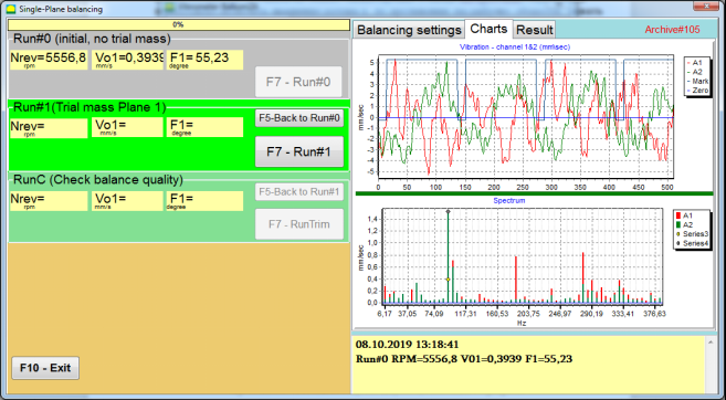
ಚಿತ್ರ 7.19. ಒಂದೇ ಸಮತಲದಲ್ಲಿ ಸಮತೋಲನ. ಆರಂಭಿಕ ರನ್ (Run#0). ಚಾರ್ಟ್ಗಳ ಟ್ಯಾಬ್
ಮಾಪನ ಪ್ರಕ್ರಿಯೆ ಮುಗಿದ ನಂತರ, ರಲ್ಲಿ Run#0 ಎಡ ಫಲಕದಲ್ಲಿ ವಿಭಾಗವು ಅಳತೆಯ ಫಲಿತಾಂಶಗಳು ಕಾಣಿಸಿಕೊಳ್ಳುತ್ತವೆ - ರೋಟರ್ ವೇಗ (RPM), RMS (Vo1) ಮತ್ತು 1x ಕಂಪನದ ಹಂತ (F1).
The "F5-Run#0 ಗೆ ಹಿಂತಿರುಗಿ” ಬಟನ್ (ಅಥವಾ F5 ಫಂಕ್ಷನ್ ಕೀ) ಅನ್ನು Run#0 ವಿಭಾಗಕ್ಕೆ ಹಿಂತಿರುಗಲು ಮತ್ತು ಅಗತ್ಯವಿದ್ದರೆ, ಕಂಪನ ನಿಯತಾಂಕಗಳನ್ನು ಅಳೆಯಲು ಪುನರಾವರ್ತಿಸಲು ಬಳಸಲಾಗುತ್ತದೆ.
Run#1 (ಟ್ರಯಲ್ ಮಾಸ್ ಪ್ಲೇನ್ 1)
Before starting the measurement of vibration parameters in the section "Run#1 (ಟ್ರಯಲ್ ಮಾಸ್ ಪ್ಲೇನ್ 1), a trial weight should be installed according "Trial weight mass" field.
ತಿಳಿದಿರುವ ಸ್ಥಳದಲ್ಲಿ (ಕೋನ) ತಿಳಿದಿರುವ ತೂಕವನ್ನು ಸ್ಥಾಪಿಸಿದಾಗ ರೋಟರ್ನ ಕಂಪನವು ಹೇಗೆ ಬದಲಾಗುತ್ತದೆ ಎಂಬುದನ್ನು ಮೌಲ್ಯಮಾಪನ ಮಾಡುವುದು ಪ್ರಾಯೋಗಿಕ ತೂಕವನ್ನು ಸ್ಥಾಪಿಸುವ ಗುರಿಯಾಗಿದೆ. ಪ್ರಯೋಗದ ತೂಕವು ಕಂಪನ ವೈಶಾಲ್ಯವನ್ನು 30% ಕಡಿಮೆ ಅಥವಾ ಆರಂಭಿಕ ವೈಶಾಲ್ಯದಿಂದ ಬದಲಾಯಿಸಬೇಕು ಅಥವಾ ಆರಂಭಿಕ ಹಂತದ 30 ಡಿಗ್ರಿ ಅಥವಾ ಅದಕ್ಕಿಂತ ಹೆಚ್ಚಿನ ಹಂತವನ್ನು ಬದಲಾಯಿಸಬೇಕು.
If it is necessary to use the "Saved coeff."ಮುಂದಿನ ಕೆಲಸಕ್ಕಾಗಿ ಸಮತೋಲನಗೊಳಿಸುವುದು, ಪ್ರಾಯೋಗಿಕ ತೂಕದ ಅನುಸ್ಥಾಪನೆಯ ಸ್ಥಳ (ಕೋನ) ಪ್ರತಿಫಲಿತ ಮಾರ್ಕ್ನ ಸ್ಥಳ (ಕೋನ) ನಂತೆಯೇ ಇರಬೇಕು.
ಬ್ಯಾಲೆನ್ಸಿಂಗ್ ಯಂತ್ರದ ರೋಟರ್ನ ತಿರುಗುವಿಕೆಯನ್ನು ಮತ್ತೊಮ್ಮೆ ಆನ್ ಮಾಡಿ ಮತ್ತು ಅದರ ತಿರುಗುವಿಕೆಯ ಆವರ್ತನವು ಸ್ಥಿರವಾಗಿದೆ ಎಂದು ಖಚಿತಪಡಿಸಿಕೊಳ್ಳಿ. ನಂತರ "" ಮೇಲೆ ಕ್ಲಿಕ್ ಮಾಡಿF7-Run#1" button (or press the F7 key on the computer keyboard).
After the measurement in the corresponding windows of the "Run#1 (ಟ್ರಯಲ್ ಮಾಸ್ ಪ್ಲೇನ್ 1)" section, the results of measuring the rotor speed (RPM), as well as the value of the RMS component (Vо1) and phase (F1) of 1x vibration appearing.
At the same time, the "Result" tab opens on the right side of the window.
ಈ ಟ್ಯಾಬ್ ದ್ರವ್ಯರಾಶಿ ಮತ್ತು ಸರಿಪಡಿಸುವ ತೂಕದ ಕೋನವನ್ನು ಲೆಕ್ಕಾಚಾರ ಮಾಡುವ ಫಲಿತಾಂಶಗಳನ್ನು ಪ್ರದರ್ಶಿಸುತ್ತದೆ, ಅಸಮತೋಲನವನ್ನು ಸರಿದೂಗಿಸಲು ರೋಟರ್ನಲ್ಲಿ ಅಳವಡಿಸಬೇಕು.
ಇದಲ್ಲದೆ, ಧ್ರುವೀಯ ನಿರ್ದೇಶಾಂಕ ವ್ಯವಸ್ಥೆಯನ್ನು ಬಳಸುವ ಸಂದರ್ಭದಲ್ಲಿ, ಪ್ರದರ್ಶನವು ದ್ರವ್ಯರಾಶಿಯ ಮೌಲ್ಯವನ್ನು ತೋರಿಸುತ್ತದೆ (M1) ಮತ್ತು ತಿದ್ದುಪಡಿ ತೂಕದ ಅನುಸ್ಥಾಪನ ಕೋನ (f1).
In the case of "Fixed positions” ಸ್ಥಾನಗಳ ಸಂಖ್ಯೆಗಳು (Zi, Zj) ಮತ್ತು ಪ್ರಯೋಗ ತೂಕದ ವಿಭಜಿತ ದ್ರವ್ಯರಾಶಿಯನ್ನು ತೋರಿಸಲಾಗುತ್ತದೆ.
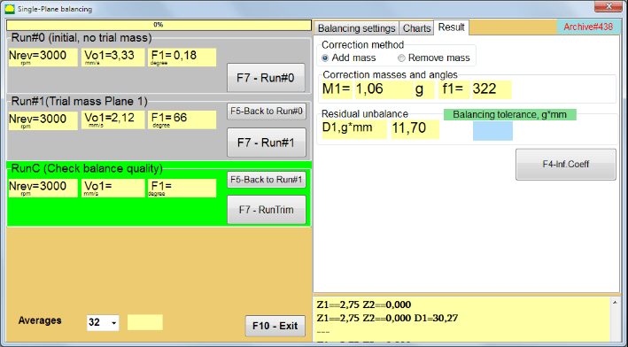
ಚಿತ್ರ 7.20. ಒಂದೇ ಸಮತಲದಲ್ಲಿ ಸಮತೋಲನ. Run#1 ಮತ್ತು ಸಮತೋಲನ ಫಲಿತಾಂಶ.
If Polar graph ಪರಿಶೀಲಿಸಲಾಗಿದೆ ಧ್ರುವ ರೇಖಾಚಿತ್ರವನ್ನು ತೋರಿಸಲಾಗುತ್ತದೆ.
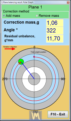
Fig. 7.21. The result of balancing. Polar graph.
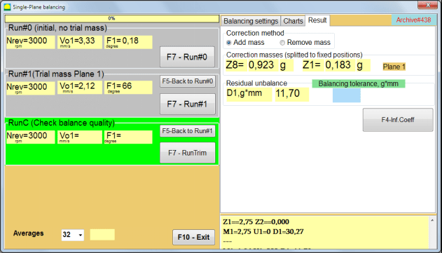
ಚಿತ್ರ 7.22. ಸಮತೋಲನದ ಫಲಿತಾಂಶ. ತೂಕವನ್ನು ವಿಭಜಿಸಲಾಗಿದೆ (ಸ್ಥಿರ ಸ್ಥಾನಗಳು)
Also if "Polar graph" was checked, Polar graph will be shown.
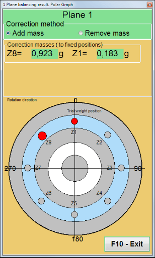
Fig. 7.23. Weight splitted on fixed positions. Polar graph
⚠️ Attention!
- 1. ಎರಡನೇ ಓಟದಲ್ಲಿ ಮಾಪನ ಪ್ರಕ್ರಿಯೆಯನ್ನು ಪೂರ್ಣಗೊಳಿಸಿದ ನಂತರ ("Run#1 (ಟ್ರಯಲ್ ಮಾಸ್ ಪ್ಲೇನ್ 1)”) ಬ್ಯಾಲೆನ್ಸಿಂಗ್ ಯಂತ್ರದ, ತಿರುಗುವಿಕೆಯನ್ನು ನಿಲ್ಲಿಸುವುದು ಮತ್ತು ಸ್ಥಾಪಿಸಲಾದ ಪ್ರಯೋಗ ತೂಕವನ್ನು ತೆಗೆದುಹಾಕುವುದು ಅವಶ್ಯಕ. ನಂತರ ಫಲಿತಾಂಶದ ಟ್ಯಾಬ್ ಡೇಟಾದ ಪ್ರಕಾರ ರೋಟರ್ನಲ್ಲಿ ಸರಿಪಡಿಸುವ ತೂಕವನ್ನು ಸ್ಥಾಪಿಸಿ (ಅಥವಾ ತೆಗೆದುಹಾಕಿ).
ಪ್ರಾಯೋಗಿಕ ತೂಕವನ್ನು ತೆಗೆದುಹಾಕದಿದ್ದರೆ, ನೀವು "" ಗೆ ಬದಲಾಯಿಸಬೇಕಾಗುತ್ತದೆBalancing settings" tab and turn on the checkbox in "ಪ್ಲೇನ್ 1 ರಲ್ಲಿ ಪ್ರಾಯೋಗಿಕ ತೂಕವನ್ನು ಬಿಡಿ". Then switch back to the "Result”ಟ್ಯಾಬ್. ತಿದ್ದುಪಡಿ ತೂಕದ ತೂಕ ಮತ್ತು ಅನುಸ್ಥಾಪನ ಕೋನವನ್ನು ಸ್ವಯಂಚಾಲಿತವಾಗಿ ಮರು ಲೆಕ್ಕಾಚಾರ ಮಾಡಲಾಗುತ್ತದೆ.
- The angular position of the corrective weight is performed from the place of installation of the trial weight. The direction of reference of the angle coincides with the direction of rotation of the rotor.
- In the case of "Fixed position" - the 1st position (Z1), coincides with the place of installation of the trial weight. The counting direction of the position number is in the direction of rotation of the rotor.
- By default the corrective weight will be added to the rotor. This is indicated by the label set in the "Add" field. If removing the weight (for example, by drilling), you must set a mark in the "Delete” field, after which the angular position of the correction weight will automatically change by 180º.
ಆಪರೇಟಿಂಗ್ ವಿಂಡೋದಲ್ಲಿ ಬ್ಯಾಲೆನ್ಸಿಂಗ್ ರೋಟರ್ನಲ್ಲಿ ತಿದ್ದುಪಡಿ ತೂಕವನ್ನು ಸ್ಥಾಪಿಸಿದ ನಂತರ (ಚಿತ್ರ 7.15 ನೋಡಿ), ರನ್ಸಿ (ಟ್ರಿಮ್) ಅನ್ನು ಕೈಗೊಳ್ಳಲು ಮತ್ತು ನಿರ್ವಹಿಸಿದ ಸಮತೋಲನದ ಪರಿಣಾಮಕಾರಿತ್ವವನ್ನು ಮೌಲ್ಯಮಾಪನ ಮಾಡುವುದು ಅವಶ್ಯಕ.
ರನ್ಸಿ (ಸಮತೋಲನ ಗುಣಮಟ್ಟವನ್ನು ಪರಿಶೀಲಿಸಿ)
⚠️ Attention! ಮಾಪನವನ್ನು ಪ್ರಾರಂಭಿಸುವ ಮೊದಲು RunC, ಯಂತ್ರದ ರೋಟರ್ನ ತಿರುಗುವಿಕೆಯನ್ನು ಆನ್ ಮಾಡುವುದು ಅವಶ್ಯಕವಾಗಿದೆ ಮತ್ತು ಅದು ಆಪರೇಟಿಂಗ್ ಮೋಡ್ (ಸ್ಥಿರ ತಿರುಗುವಿಕೆಯ ಆವರ್ತನ) ಪ್ರವೇಶಿಸಿದೆ ಎಂದು ಖಚಿತಪಡಿಸಿಕೊಳ್ಳಿ.
To perform vibration measurement in the "ರನ್ಸಿ (ಸಮತೋಲನ ಗುಣಮಟ್ಟವನ್ನು ಪರಿಶೀಲಿಸಿ)" section, click on the "F7 – RunTrim" button (or press the F7 key on the keyboard).
Upon successful completion of the measurement process, in the "ರನ್ಸಿ (ಸಮತೋಲನ ಗುಣಮಟ್ಟವನ್ನು ಪರಿಶೀಲಿಸಿ)" section in the left panel, the results of measuring the rotor speed (RPM) appear, as well as the value of the RMS component (Vo1) and phase (F1) of 1x vibration.
In the "Result” ಟ್ಯಾಬ್, ಹೆಚ್ಚುವರಿ ಸರಿಪಡಿಸುವ ತೂಕದ ದ್ರವ್ಯರಾಶಿ ಮತ್ತು ಅನುಸ್ಥಾಪನ ಕೋನವನ್ನು ಲೆಕ್ಕಾಚಾರ ಮಾಡುವ ಫಲಿತಾಂಶಗಳನ್ನು ಪ್ರದರ್ಶಿಸಲಾಗುತ್ತದೆ.
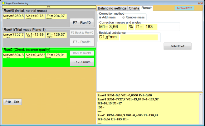
ಚಿತ್ರ 7.24. ಒಂದೇ ಸಮತಲದಲ್ಲಿ ಸಮತೋಲನ. ರನ್ ಟ್ರಿಮ್ ಅನ್ನು ನಿರ್ವಹಿಸುವುದು. ಫಲಿತಾಂಶ ಟ್ಯಾಬ್
ಉಳಿದಿರುವ ಅಸಮತೋಲನವನ್ನು ಸರಿದೂಗಿಸಲು ರೋಟರ್ನಲ್ಲಿ ಈಗಾಗಲೇ ಜೋಡಿಸಲಾದ ತಿದ್ದುಪಡಿ ತೂಕಕ್ಕೆ ಈ ತೂಕವನ್ನು ಸೇರಿಸಬಹುದು. ಹೆಚ್ಚುವರಿಯಾಗಿ, ಸಮತೋಲನದ ನಂತರ ಸಾಧಿಸಿದ ಉಳಿದ ರೋಟರ್ ಅಸಮತೋಲನವನ್ನು ಈ ವಿಂಡೋದ ಕೆಳಗಿನ ಭಾಗದಲ್ಲಿ ಪ್ರದರ್ಶಿಸಲಾಗುತ್ತದೆ.
ಸಮತೋಲಿತ ರೋಟರ್ನ ಉಳಿದ ಕಂಪನ ಮತ್ತು / ಅಥವಾ ಉಳಿದ ಅಸಮತೋಲನದ ಪ್ರಮಾಣವು ತಾಂತ್ರಿಕ ದಾಖಲಾತಿಯಲ್ಲಿ ಸ್ಥಾಪಿಸಲಾದ ಸಹಿಷ್ಣುತೆಯ ಅವಶ್ಯಕತೆಗಳನ್ನು ಪೂರೈಸಿದಾಗ, ಸಮತೋಲನ ಪ್ರಕ್ರಿಯೆಯನ್ನು ಪೂರ್ಣಗೊಳಿಸಬಹುದು.
Otherwise, the balancing process may continue. This allows the method of successive approximations to correct possible errors that may occur during the installation (removal) of the corrective weight on a balanced rotor.
ಬ್ಯಾಲೆನ್ಸಿಂಗ್ ರೋಟರ್ನಲ್ಲಿ ಸಮತೋಲನ ಪ್ರಕ್ರಿಯೆಯನ್ನು ಮುಂದುವರಿಸುವಾಗ, ಹೆಚ್ಚುವರಿ ಸರಿಪಡಿಸುವ ದ್ರವ್ಯರಾಶಿಯನ್ನು ಸ್ಥಾಪಿಸುವುದು (ತೆಗೆದುಹಾಕುವುದು) ಅವಶ್ಯಕವಾಗಿದೆ, ಅದರ ನಿಯತಾಂಕಗಳನ್ನು ವಿಭಾಗದಲ್ಲಿ ಸೂಚಿಸಲಾಗುತ್ತದೆ "ತಿದ್ದುಪಡಿ ದ್ರವ್ಯರಾಶಿಗಳು ಮತ್ತು ಕೋನಗಳು".
ಪ್ರಭಾವ ಗುಣಾಂಕಗಳು (1-ಪ್ಲೇನ್)
The "F4-Inf.Coeff" button in the "Result" tab is used to view and store in the computer memory the coefficients of rotor balancing (Influence coefficients) calculated from the results of calibration runs.
When it is pressed, the "ಪ್ರಭಾವ ಗುಣಾಂಕಗಳು (ಏಕ ಸಮತಲ)" window appears on the computer display, in which balancing coefficients calculated from the results of calibration (test) runs are displayed. If during the subsequent balancing of this machine it is supposed to use the "Saved coeff.” ಮೋಡ್, ಈ ಗುಣಾಂಕಗಳನ್ನು ಕಂಪ್ಯೂಟರ್ ಮೆಮೊರಿಯಲ್ಲಿ ಸಂಗ್ರಹಿಸಬೇಕು.
To do this, click the "F9 - Save" button and go to the second page of the "Influence coeff. archive. Single plane."

ಚಿತ್ರ 7.25. 1 ನೇ ಸಮತಲದಲ್ಲಿ ಸಮತೋಲನ ಗುಣಾಂಕಗಳು
ನಂತರ ನೀವು ಈ ಯಂತ್ರದ ಹೆಸರನ್ನು ನಮೂದಿಸಬೇಕು "ರೋಟರ್" column and click "F2-ಉಳಿಸಿಕಂಪ್ಯೂಟರ್ನಲ್ಲಿ ನಿರ್ದಿಷ್ಟಪಡಿಸಿದ ಡೇಟಾವನ್ನು ಉಳಿಸಲು ಬಟನ್.
ನಂತರ ನೀವು " ಅನ್ನು ಒತ್ತುವ ಮೂಲಕ ಹಿಂದಿನ ವಿಂಡೋಗೆ ಹಿಂತಿರುಗಬಹುದುF10-ನಿರ್ಗಮನ" button (or the F10 function key on the computer keyboard).
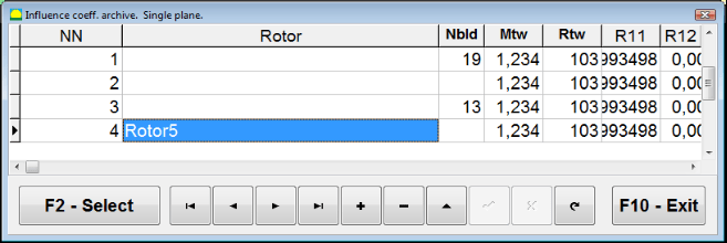
Fig. 7.26. "Influence coeff. archive. Single plane."
ಸಮತೋಲನ ವರದಿ
ಉಳಿಸಿದ ಎಲ್ಲಾ ಡೇಟಾವನ್ನು ಸಮತೋಲನಗೊಳಿಸಿದ ನಂತರ ಮತ್ತು ಬ್ಯಾಲೆನ್ಸಿಂಗ್ ವರದಿಯನ್ನು ರಚಿಸಲಾಗಿದೆ. ಅಂತರ್ನಿರ್ಮಿತ ಸಂಪಾದಕದಲ್ಲಿ ನೀವು ವರದಿಯನ್ನು ವೀಕ್ಷಿಸಬಹುದು ಮತ್ತು ಸಂಪಾದಿಸಬಹುದು. ರಲ್ಲಿ "Balancing archive in one plane" (Fig. 7.9) press button "F9 -ವರದಿ" to access to the balancing report editor.
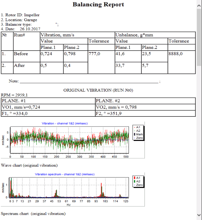
Fig. 7.27. Balancing report.
ಉಳಿಸಿದ ಕೋಫ್. 1 ಸಮತಲದಲ್ಲಿ ಉಳಿಸಿದ ಪ್ರಭಾವದ ಗುಣಾಂಕಗಳೊಂದಿಗೆ ಸಮತೋಲನ ಪ್ರಕ್ರಿಯೆ.
Setting up the measuring system (input of initial data).
Saved coeff. balancing ಬ್ಯಾಲೆನ್ಸಿಂಗ್ ಗುಣಾಂಕಗಳನ್ನು ಈಗಾಗಲೇ ನಿರ್ಧರಿಸಿದ ಮತ್ತು ಕಂಪ್ಯೂಟರ್ ಮೆಮೊರಿಗೆ ಪ್ರವೇಶಿಸಿದ ಯಂತ್ರದಲ್ಲಿ ನಿರ್ವಹಿಸಬಹುದು.
⚠️ Attention! ಉಳಿಸಿದ ಗುಣಾಂಕಗಳೊಂದಿಗೆ ಸಮತೋಲನ ಮಾಡುವಾಗ, ಕಂಪನ ಸಂವೇದಕ ಮತ್ತು ಹಂತದ ಕೋನ ಸಂವೇದಕವನ್ನು ಆರಂಭಿಕ ಸಮತೋಲನದ ಸಮಯದಲ್ಲಿ ಅದೇ ರೀತಿಯಲ್ಲಿ ಸ್ಥಾಪಿಸಬೇಕು.
ಆರಂಭಿಕ ಡೇಟಾದ ಇನ್ಪುಟ್ Saved coeff. balancing (as in the case of primary("New rotor") balancing) begins in the "ಏಕ ಸಮತಲ ಸಮತೋಲನ. ಸಮತೋಲನ ಸೆಟ್ಟಿಂಗ್ಗಳು.".
In this case, in the "Influence coefficients" section, select the "ಉಳಿಸಿದ ಕೋಫ್" item. In this case, the second page of the "ಪ್ರಭಾವ ಕೋಫ್. ಆರ್ಕೈವ್. ಏಕ ವಿಮಾನ.", which stores an archive of the saved balancing coefficients.
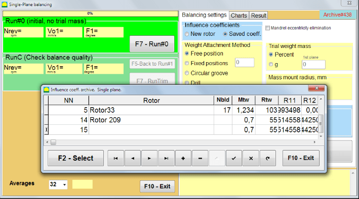
ಚಿತ್ರ 7.28. 1 ಸಮತಲದಲ್ಲಿ ಉಳಿಸಿದ ಪ್ರಭಾವದ ಗುಣಾಂಕಗಳೊಂದಿಗೆ ಸಮತೋಲನಗೊಳಿಸುವುದು
Moving through the table of this archive using the "►" or "◄" control buttons, you can select the desired record with balancing coefficients of the machine of interest to us. Then, to use this data in current measurements, press the "F2 - ಆಯ್ಕೆಮಾಡಿ" button.
After that, the contents of all other windows of the “ಏಕ ಸಮತಲ ಸಮತೋಲನ. ಸಮತೋಲನ ಸೆಟ್ಟಿಂಗ್ಗಳು." are filled in automatically.
ಆರಂಭಿಕ ಡೇಟಾದ ಇನ್ಪುಟ್ ಅನ್ನು ಪೂರ್ಣಗೊಳಿಸಿದ ನಂತರ, ನೀವು ಅಳೆಯಲು ಪ್ರಾರಂಭಿಸಬಹುದು.
Measurements during balancing with saved influence coefficients
ಉಳಿಸಿದ ಪ್ರಭಾವದ ಗುಣಾಂಕಗಳೊಂದಿಗೆ ಸಮತೋಲನವು ಕೇವಲ ಒಂದು ಆರಂಭಿಕ ರನ್ ಮತ್ತು ಸಮತೋಲನ ಯಂತ್ರದ ಕನಿಷ್ಠ ಒಂದು ಪರೀಕ್ಷಾ ರನ್ ಅಗತ್ಯವಿರುತ್ತದೆ.
⚠️ Attention! ಮಾಪನವನ್ನು ಪ್ರಾರಂಭಿಸುವ ಮೊದಲು, ರೋಟರ್ನ ತಿರುಗುವಿಕೆಯನ್ನು ಆನ್ ಮಾಡುವುದು ಮತ್ತು ತಿರುಗುವ ಆವರ್ತನವು ಸ್ಥಿರವಾಗಿದೆ ಎಂದು ಖಚಿತಪಡಿಸಿಕೊಳ್ಳಿ.
To carry out the measurement of vibration parameters in the "Run#0 (ಆರಂಭಿಕ, ಪ್ರಾಯೋಗಿಕ ದ್ರವ್ಯರಾಶಿ ಇಲ್ಲ)" section, press "F7 – Run#0" (or press the F7 key on the computer keyboard).
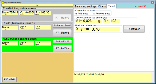
ಚಿತ್ರ 7.29. ಒಂದು ಸಮತಲದಲ್ಲಿ ಉಳಿಸಿದ ಪ್ರಭಾವದ ಗುಣಾಂಕಗಳೊಂದಿಗೆ ಸಮತೋಲನ. ಒಂದು ರನ್ ನಂತರ ಫಲಿತಾಂಶಗಳು.
In the corresponding fields of "Run#0" section, the results of measuring the rotor speed (RPM), the value of the RMS component (Vо1) and phase (F1) of 1x vibration appear.
At the same time, the "Resultಈ ಟ್ಯಾಬ್ ದ್ರವ್ಯರಾಶಿ ಮತ್ತು ಸರಿಪಡಿಸುವ ತೂಕದ ಕೋನವನ್ನು ಲೆಕ್ಕಾಚಾರ ಮಾಡುವ ಫಲಿತಾಂಶಗಳನ್ನು ಪ್ರದರ್ಶಿಸುತ್ತದೆ, ಅಸಮತೋಲನವನ್ನು ಸರಿದೂಗಿಸಲು ರೋಟರ್ನಲ್ಲಿ ಅಳವಡಿಸಬೇಕು.
Moreover, in the case of using a polar coordinate system, the display shows the mass values and the installation angles of the correction weights.
ಸ್ಥಿರ ಸ್ಥಾನಗಳ ಮೇಲೆ ಸರಿಪಡಿಸುವ ತೂಕದ ವಿಭಜನೆಯ ಸಂದರ್ಭದಲ್ಲಿ, ಬ್ಯಾಲೆನ್ಸಿಂಗ್ ರೋಟರ್ನ ಸ್ಥಾನಗಳ ಸಂಖ್ಯೆಗಳು ಮತ್ತು ಅವುಗಳ ಮೇಲೆ ಸ್ಥಾಪಿಸಬೇಕಾದ ತೂಕದ ದ್ರವ್ಯರಾಶಿಯನ್ನು ಪ್ರದರ್ಶಿಸಲಾಗುತ್ತದೆ.
ಇದಲ್ಲದೆ, ವಿಭಾಗ 7.4.2 ರಲ್ಲಿ ಸೂಚಿಸಲಾದ ಶಿಫಾರಸುಗಳಿಗೆ ಅನುಗುಣವಾಗಿ ಸಮತೋಲನ ಪ್ರಕ್ರಿಯೆಯನ್ನು ಕೈಗೊಳ್ಳಲಾಗುತ್ತದೆ. ಪ್ರಾಥಮಿಕ ಸಮತೋಲನಕ್ಕಾಗಿ.
Mandrel eccentricity elimination (Index balancing)
If during balancing the rotor is installed in a cylindrical mandrel, then the eccentricity of the mandrel may introduce an additional error. To eliminate this error, the rotor should be deployed in the mandrel 180 degrees and carry out an additional start. This is called index balancing.
To carry out index balancing, a special option is provided in the Balanset-1A program. When checked Mandrel eccentricity elimination an additional RunEcc section appears in the balancing window.

ಚಿತ್ರ 7.30. ಸೂಚ್ಯಂಕ ಸಮತೋಲನಕ್ಕಾಗಿ ಕೆಲಸ ಮಾಡುವ ವಿಂಡೋ.
ರನ್ # 1 (ಟ್ರಯಲ್ ಮಾಸ್ ಪ್ಲೇನ್ 1) ಅನ್ನು ಚಲಾಯಿಸಿದ ನಂತರ, ಒಂದು ವಿಂಡೋ ಕಾಣಿಸಿಕೊಳ್ಳುತ್ತದೆ
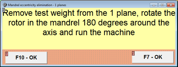
ಚಿತ್ರ 7.31 ಸೂಚ್ಯಂಕ ಸಮತೋಲನ ಗಮನ ವಿಂಡೋ.
After installing the rotor with an 180 turn, Run Ecc must be completed. The program will automatically calculate the true rotor imbalance without affecting the mandrel eccentricity.
7.5 Two plane balancing
Before starting work in the Two plane balancing mode, it is necessary to install vibration sensors on the machine body at the selected measurement points and connect them to the inputs X1 and X2 of the measuring unit, respectively.
An optical phase angle sensor must be connected to input X3 of the measuring unit. In addition, to use this sensor, a reflective tape must be glued onto the accessible rotor surface of the balancing machine.
Detailed requirements for choosing the installation location of sensors and their mounting at the facility during balancing are set out in Appendix 1.
The work on the program in the "Two plane balancing" mode starts from the Main window of the programs.
Click on the "F3-Two plane" button (or press the F3 key on the computer keyboard).
Further, click on the “F7 – Balancing” button, after which a working window will appear on the computer display (see Fig. 7.13), selection of the archive for saving data when balancing in two p
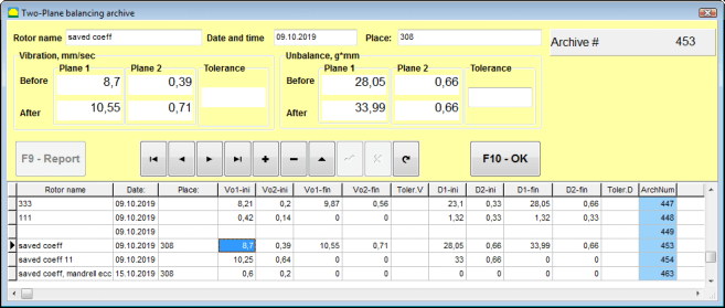
Fig. 7.32 Two plane balancing archive window.
In this window you need to enter the data of the balanced rotor. After pressing the “F10-OK" button, a balancing window will appear.
Balancing settings (2-plane)
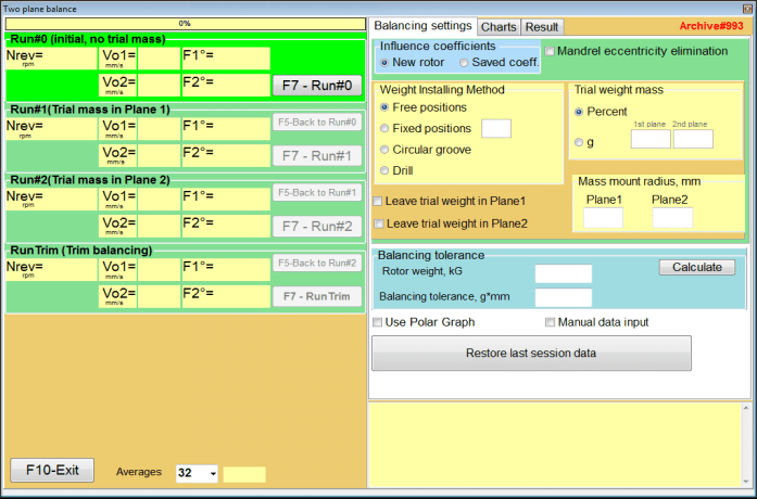
Fig. 7.33. Balancing in two planes window.
On the right side of the window is the "Balancing settings" tab for entering settings before balancing.
- Influence coefficients Balancing a new rotor or balancing using stored influence coefficients (balancing coefficients)
- Mandrel eccentricity elimination - Balancing with additional start to eliminate the influence of the eccentricity of the mandrel
- Weight Attachment Method Installation of corrective weights in an arbitrary place on the circumference of the rotor or in a fixed position. Calculations for drilling when removing the mass.
- "Free position" - weights can be installed in an arbitrary angular positions on the circumference of the rotor.
- "Fixed position” – weight can be installed in fixed angular positions on the rotor, for example, on blades or holes (for example 12 holes – 30 degrees), etc. The number of fixed positions must be entered in the appropriate field. After balancing, the program will automatically split the weight into two parts and indicate the number of positions on which it is necessary to establish the masses obtained.
- Trial weight mass - Trial weight
- Leave trial weight in Plane1 / Plane2 - Remove or leave trial weight when balancing.
- Mass mount radius, mm - Radius of mounting trial and corrective weights
- Balancing tolerance Entering or calculating residual imbalance tolerances in g-mm
- Use Polar Graph - Use polar graph to display balancing results
- Manual data input - Manual data entry for calculating balancing weights
- Restore last session data - Recovery of the measurement data of the last session in the event of failure to continue balancing.
2 planes balancing. New rotor
Setting up the measuring system (input of initial data).
Input of the initial data for the New rotor balancing in the "Two plane balancing. Settings".
In this case, in the "Influence coefficients" section, select the "New rotor" item.
Further, in the section "Trial weight mass", you must select the unit of measurement of the mass of the trial weight - "Gram" or "Percent".
When choosing the unit of measure "Percent”, all further calculations of the mass of the corrective weight will be performed as a percentage in relation to the mass of the trial weight.
When choosing the "Gram” unit of measurement, all further calculations of the mass of the corrective weight will be performed in grams. Then enter in the windows located to the right of the inscription “Gram" the mass of trial weights that will be installed on the rotor.
⚠️ Attention! If it is necessary to use the "Saved coeff.” Mode for further work during initial balancing, the mass of trial weights must be entered in grams.
Then select "Weight Attachment Method" - "Circum" or "Fixed position".
If you select "Fixed position", you must enter the number of positions.
Calculation of tolerance for residual imbalance (Balancing tolerance)
The tolerance for residual imbalance (Balancing tolerance) can be calculated in accordance with the procedure described in ISO 1940 Vibration. Balance quality requirements for rotors in a constant (rigid) state. Part 1. Specification and verification of balance tolerances.

ಚಿತ್ರ 7.34. ಬ್ಯಾಲೆನ್ಸಿಂಗ್ ಟಾಲರೆನ್ಸ್ ಲೆಕ್ಕಾಚಾರ ವಿಂಡೋ
Initial run (Run#0)
When balancing in two planes in the "New rotor” mode, balancing requires three calibration runs and at least one test run of the balancing machine.
The vibration measurement at the first start of the machine is performed in the "Two plane balance" working window in the "Run#0" section.
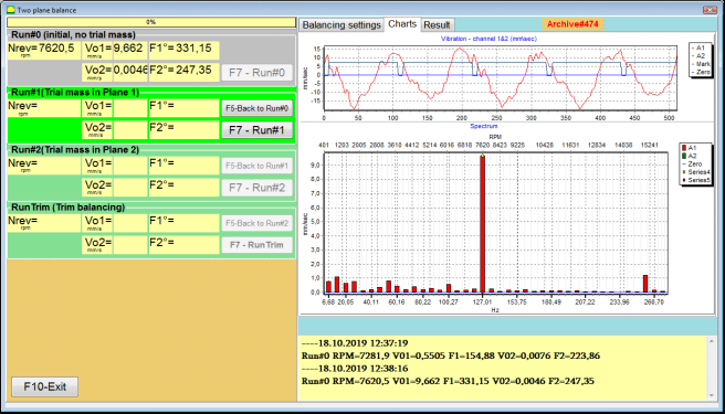
Fig. 7.35. Measurement results at balancing in two planes after the initial run.
⚠️ Attention! Before starting the measurement, it is necessary to turn on the rotation of the rotor of the balancing machine and make sure that it has entered the operating mode with a stable speed.
To measure vibration parameters in the Run#0 section, click on the "F7 – Run#0" button (or press the F7 key on a computer keyboard)
The results of measuring the rotor speed (RPM), the value RMS (VО1, VО2) and phases (F1, F2) of 1x vibration appearing appear in the corresponding windows of the Run#0 section.
Run#1.Trial mass in Plane1
Before starting to measure vibration parameters in the "Run#1.Trial mass in Plane1” section, you should stop the rotation of the rotor of the balancing machine and install a trial weight on it, the mass selected in the “Trial weight mass" section.
⚠️ Attention!
- 1. The question of choosing the mass of trial weights and their installation places on the rotor of a balancing machine is discussed in detail in Appendix 1.
- If it is necessary to use the Saved coeff. Mode in future work, the place for installing the trial weight must necessarily coincide with the place for installing the mark used to read the phase angle.
After this, it is necessary to turn on the rotation of the rotor of the balancing machine again and make sure that it has entered the operating mode.
To measure vibration parameters in the "Run # 1.Trial mass in Plane1" section, click on the "F7 – Run#1" button (or press the F7 key on the computer keyboard).
Upon successful completion of the measurement process, you are returned to the tab of measurement results.
In this case, in the corresponding windows of the "Run#1. Trial mass in Plane1” section, the results of measuring the rotor speed (RPM), as well as the value of the components of the RMS (Vо1, Vо2) and phases (F1, F2) of 1x vibration.
"Run # 2.Trial mass in Plane2"
Before starting to measure vibration parameters in the section "Run # 2.Trial mass in Plane2", you must perform the following steps:
- stop the rotation of the rotor of the balancing machine;
- remove the trial weight installed in plane 1;
- install a trial weight in plane 2, the mass selected in the section "Trial weight mass".
After this, turn on the rotation of the rotor of the balancing machine and make sure that it has entered the operating speed.
To begin the measurement of vibration in the "Run # 2.Trial mass in Plane2" section, click on the "F7 – Run # 2" button (or press the F7 key on the computer keyboard). Then the "Result" tab opens.
In the case of using the Weight Attachment Method" - "Free positions, the display shows the mass values (M1, M2) and installation angles (f1, f2) of the corrective weights.
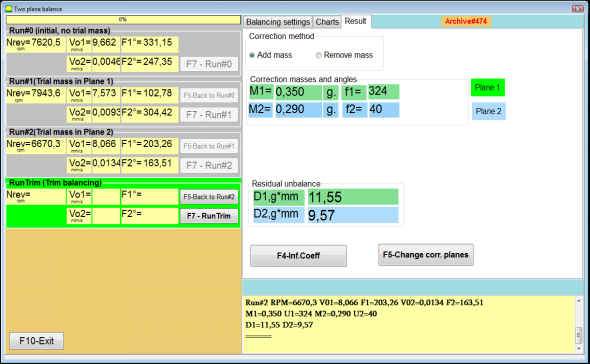
Fig. 7.36. Results of calculation of corrective weights – free position
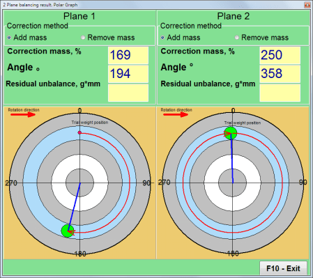
Fig. 7.37. Results of calculation of corrective weights – free position. Polar diagram
In the case of using the Weight Attachment Method" – "Fixed positions

Fig. 7.38. Results of calculation of corrective weights – fixed position.
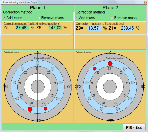
Fig. 7.39. Results of calculation of corrective weights – fixed position. Polar diagram.
In the case of using the Weight Attachment Method" – "Circular groove"
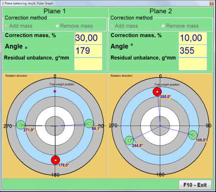
Fig. 7.40. Results of calculation of corrective weights – Circular groove.
⚠️ Attention!
- After completing the measurement process on the RUN#2 of the balancing machine, stop the rotation of the rotor and remove the trial weight previously installed. Then you can to install (or remove) corrective weights.
- The angular position of the corrective weights in the polar coordinate system is counted from the place of installation of the trial weight in the direction of rotation of the rotor.
- In the case of "Fixed position" - the 1st position (Z1), coincides with the place of installation of the trial weight. The counting direction of the position number is in the direction of rotation of the rotor.
- By default the corrective weight will be added to the rotor. This is indicated by the label set in the "Add" field. If removing the weight (for example, by drilling), you must set a mark in the "Delete” field, after which the angular position of the correction weight will automatically change by 180º.
RunC (Trim run)
After installing the correction weight on the balancing rotor it is necessary to carry out a RunC (trim) and evaluate the effectiveness of the performed balancing.
⚠️ Attention! Before starting the measurement at the test run, it is necessary to turn on the rotation of the rotor of the machine and make sure that it has entered the operating
To measure vibration parameters in the RunTrim (Check balance quality) section, click on the "F7 – RunTrim" button (or press the F7 key on the computer keyboard).
The results of measuring the rotor rotation frequency (RPM), as well as the value of the RMS component (Vо1) and phase (F1) of 1x vibration will be shown.
The "Result" tab appears on right side of the working window with the table of measurement results, which displays the results of calculating the parameters of additional corrective weights.
These weights can be added to corrective weights that are already installed on the rotor to compensate for residual imbalance.
In addition, the residual rotor unbalance achieved after balancing is displayed in the lower part of this window.
In the case when the values of the residual vibration and / or residual unbalance of the balanced rotor satisfy the tolerance requirements established in the technical documentation, the balancing process can be completed.
Otherwise, the balancing process may continue. This allows the method of successive approximations to correct possible errors that may occur during the installation (removal) of the corrective weight on a balanced rotor.
When continuing the balancing process on the balancing rotor, it is necessary to install (remove) additional corrective mass, the parameters of which are indicated in the “Result” window.
In the "Result" window there are two control buttons can be used - "F4-Inf.Coeff", "F5 – Change correction planes".
Influence coefficients (2 planes)
The "F4-Inf.Coeff" button (or the F4 function key on the computer keyboard) is used to view and save rotor balancing coefficients in the computer memory, calculated from the results of two calibration starts.
When it is pressed, the "Influence coefficients (two planes)" working window appears on the computer display, in which balancing coefficients calculated based on the results of the first three calibration starts are displayed.

Fig. 7.41. Working window with balancing coefficients in 2 planes.
In the future, when balancing of such type of the machine it is supposed, require to use the “Saved coeff." mode and balancing coefficients stored in the computer memory.
To save coefficients, click the "F9 – Save" button and go to the "Influence coefficients archive (2planes)" windows (see Fig. 7.42)
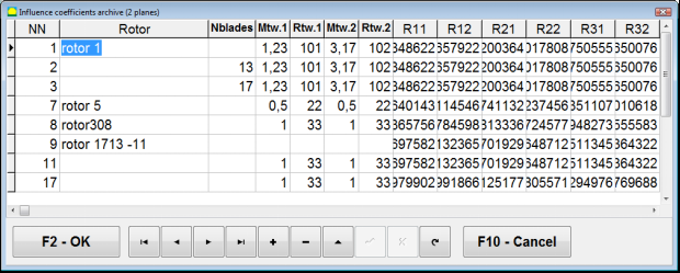
Fig. 7.42. The second page of the working window with balancing coefficients in 2 planes.
Change correction planes
The "F5 – Change correction planes" button is used when require change the position of the correction planes, when it is necessary to recalculate the masses and installation angles corrective weights.
This mode is primarily useful when balancing rotors of complex shape (for example, crankshafts).
When this button is pressed, the working window "Recalculation of correction weights mass and angle to other correction planes" is displayed on the computer display.
In this working window, you should select one of the 4 possible options by clicking corresponding picture.
The original correction planes (Н1 and Н2) in Fig. 7.29 are marked in green, and new (K1 and K2), for which it recounts, in red.
Then, in the "Calculation data" section, enter the requested data, including:
- the distance between the corresponding correction planes (a, b, c);
- new values of the radii of the installation of corrective weights on the rotor (R1 ', R2').
After entering the data, you must press the button "F9-calculate"
The calculation results (masses M1, M2 and installation angles of corrective weights f1, f2) are displayed in the corresponding section of this working window (see Fig. 7.42).
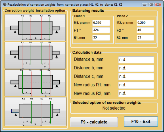
Fig. 7.43 Change correction planes. Recalculation of correction mass and angle to other correction planes.
Saved coeff. balancing in 2 planes
Saved coeff. balancing can be performed on a machine for which balancing coefficients have already been determined and saved in the computer memory.
⚠️ Attention! When re-balancing, the vibration sensors and the phase angle sensor must be installed in the same way as during the initial balancing.
Input of initial data for re-balancing begins in the "Two plane balance. Balancing settings".
In this case, in the "Influence coefficients" section, select the "Saved coeff." Item. In this case, the window "Influence coefficients archive (2planes)" will appear, in which the archive of the previously determined balancing coefficients is stored.
Moving through the table of this archive using the "►" or "◄" control buttons, you can select the desired record with balancing coefficients of the machine of interest to us. Then, to use this data in current measurements, press the "F2 – OK” button and return to the previous working window.
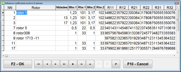
Fig. 7.44. The second page of the working window with balancing coefficients in 2 planes.
After that, the contents of all other windows of the “Balancing in 2 pl. Source data" is filled in automatically.
Saved coeff. Balancing
"Saved coeff.” balancing requires only one tuning start and at least one test start of the balancing machine.
Vibration measurement at the tuning start (Run # 0) of the machine is performed in the "Balancing in 2 planes" working window with a table of balancing results in the Run # 0 section.
⚠️ Attention! Before starting the measurement, it is necessary to turn on the rotation of the rotor of the balancing machine and make sure that it has entered the operating mode with a stable speed.
To measure vibration parameters in the Run # 0 section, click the "F7 – Run#0" button (or press the F7 key on the computer keyboard).
The results of measuring the rotor speed (RPM), as well as the value of the components of the RMS (VО1, VО2) and phases (F1, F2) of the 1x vibration appear in the corresponding fields of the Run # 0 section.
At the same time, the "Result" tab opens, which displays the results of calculating the parameters of corrective weights that must be installed on the rotor to compensate for its imbalance.
Moreover, in the case of using the polar coordinate system, the display shows the mass values and installation angles of corrective weights.
In the case of decomposition of corrective weights on the blades, the numbers of the blades of the balancing rotor and the mass of weight that need to be installed on them are displayed.
Further, the balancing process is carried out in accordance with the recommendations set out in section 7.6.1.2. for primary balancing.
⚠️ Attention!
- After completion of the measurement process after the second start of the balanced machine stop the rotation of its rotor and remove the previously set trial weight. Only then you can begin to install (or remove) correction weight on the rotor.
- Counting the angular position of the place of adding (or removing) of the correction weight from the rotor is carried out on the installation site of trial weight in the polar coordinate system. Counting direction coincides with the direction of the angle of rotor rotation.
- In case of balancing on the blades – the balanced rotor blade, designated as position 1, coincides with the place of the trial weight installation. Reference number direction of the blade shown on the computer display is performed in the direction of the rotor rotation.
- In this version of the program it is accepted by default that correction weight will be added on the rotor. The tag established in the field "Addition" testifies to it. In case of correction of imbalance by removal of a weight (for example by drilling) it is necessary to establish tag in the field "Removal" then the angular position of the correction weight will change automatically on 180º.
Mandrel eccentricity elimination (Index balancing) - Two Planes
If during balancing the rotor is installed in a cylindrical mandrel, then the eccentricity of the mandrel may introduce an additional error. To eliminate this error, the rotor should be deployed in the mandrel 180 degrees and carry out an additional start. This is called index balancing.
To carry out index balancing, a special option is provided in the Balanset-1A program. When checked Mandrel eccentricity elimination an additional RunEcc section appears in the balancing window.
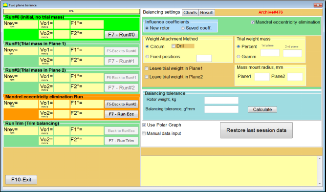
Fig. 7.45. The working window for Index balancing.
After running Run # 2 (Trial mass Plane 2), a window will appear
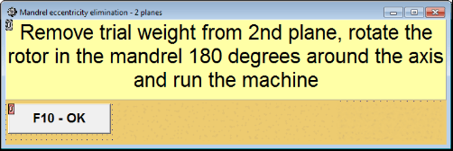
Fig. 7.46. Attention windows
After installing the rotor with an 180 turn, Run Ecc must be completed. The program will automatically calculate the true rotor imbalance without affecting the mandrel eccentricity.
7.6 Charts mode
Working in the "Charts" mode begins from the Initial window (see. Fig. 7.1) by pressing "F8 – Charts". Then opens a window "Measurement of vibration on two channels. Charts" (see. Fig. 7.19).

Fig. 7.47. Operating window "Measurement of vibration on two channels. Charts".
While working in this mode it is possible to plot four versions of vibration chart.
The first version allows to get a timeline function of the overall vibration (of vibration velocity) on the first and second measuring channels.
The second version allows you to get graphs of vibration (of vibration velocity), which occurs on rotation frequency and its higher harmonical components.
These graphs are obtained as a result of the synchronous filtering of the overall vibration time function.
The third version provides vibration charts with the results of the harmonical analysis.
The fourth version allows to get a vibration chart with the results of the spectrum analysis.
Charts of overall vibration
To plot a overall vibration chart in the operating window "Measurement of vibration on two channels. Charts" it is necessary to select the operating mode "overall vibration” by clicking the appropriate button. Then set the measurement of vibration in the box “Duration, in seconds,” by clicking on the button «▼» and select from the drop-down list the desired duration of the measurement process, which may be equal to 1, 5, 10, 15 or 20 seconds;
Upon readiness press (click) the "F9-Measure" button then the vibration measurement process begins simultaneously on two channels.
After completion of the measurement process in the operating window appear charts of time function of the overall vibration of the first (red) and the second (green) channels (see. Fig. 7.47).
On these charts time is plotted on X-axis and the amplitude of the vibration velocity (mm/sec) is plotted on Y-axis.
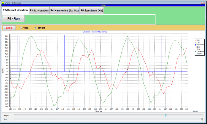
Fig. 7.48. Operating window for the output of the time function of the overall vibration charts
There are also marks (blue-colored) in these graphs connecting charts of overall vibration with the rotation frequency of the rotor. In addition, each mark indicates beginning (end) of the next revolution of the rotor.
In need of the scale change of the chart on X-axis the slider, pointed by an arrow on fig. 7.20, can be used.
Charts of 1x vibration
To plot a 1x vibration chart in the operating window "Measurement of vibration on two channels. Charts" it is necessary to select the operating mode "1x vibration" by clicking the appropriate button.
Then appears operating window "1x vibration".
Press (click) the "F9-Measure" button then the vibration measurement process begins simultaneously on two channels.
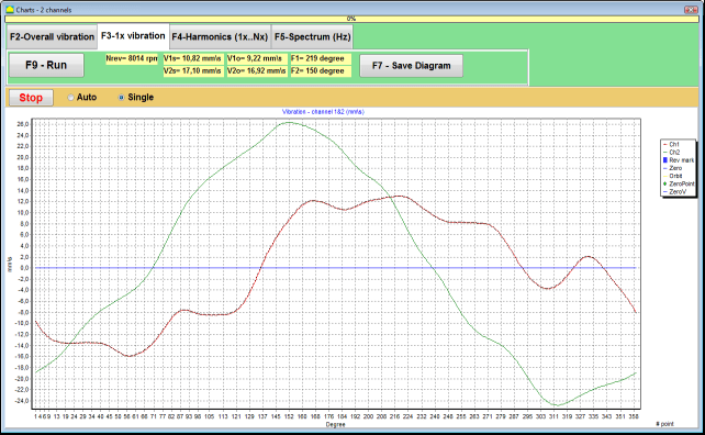
Fig. 7.49. Operating window for the output of the 1x vibration charts.
After completion of the measurement process and mathematical calculation of results (synchronous filtering of the time function of the overall vibration) on display in the main window on a period equal to one revolution of the rotor appear charts of the 1x vibration on two channels.
In this case, a chart for the first channel is depicted in red and for the second channel in green. On these charts angle of the rotor revolution is plotted (from mark to mark) on X-axis and the amplitude of the vibration velocity (mm/sec) is plotted on Y-axis.
In addition, in the upper part of the working window (to the right of the button “F9 – Measure") numerical values of vibration measurements of both channels, similar to those we get in the "Vibration meter" mode, are displayed.
In particular: RMS value of the overall vibration (V1s, V2s), the magnitude of RMS (V1o, V2o) and phase (Fi, Fj) of the 1x vibration and rotor speed (Nrev).
Vibration charts with the results of harmonical analysis
To plot a chart with the results of harmonical analysis in the operating window "Measurement of vibration on two channels. Charts" it is necessary to select the operating mode "Harmonical analysis" by clicking the appropriate button.
Then appears an operating window for simultaneous output of charts of temporary function and of spectrum of vibration harmonical aspects whose period is equal or multiple to the rotor rotation frequency (see Fig. 7.49)
ಗಮನ!
When operating in this mode it is necessary to use the phase angle sensor which synchronizes the measurement process with the rotor frequency of the machines to which the sensor is set.
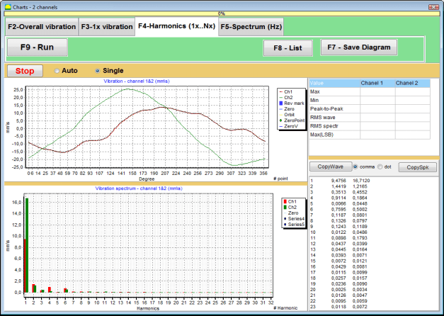
Fig. 7.50. Operating window harmonics of 1x vibration.
Upon readiness press (click) the "F9-Measure" button then the vibration measurement process begins simultaneously on two channels.
After completion of the measurement process in operating window appear charts of time function (higher chart) and harmonics of 1x vibration (lower chart).
The number of harmonic components is plotted on X-axis and RMS of the vibration velocity (mm/sec) is plotted on Y-axis.
Charts of vibration time domain and spectrum
To plot a spectrum chart use "F5-Spectrum" tab:
Then appears an operating window for simultaneous output of charts of wave and spectrum of vibration.

Fig. 7.51. Operating window for the output of the spectrum of vibration.
Upon readiness press (click) the "F9-Measure" button then the vibration measurement process begins simultaneously on two channels.
After completion of the measurement process in operating window appear charts of time function (higher chart) and spectrum of vibration (lower chart).
The vibration frequency is plotted on X-axis and RMS of the vibration velocity (mm/sec) is plotted on Y-axis.
In this case, a chart for the first channel is depicted in red and for the second channel in green.
General instructions on operation and maintenance of the device
8.1 Balancing Quality Criteria (ISO 2372 Standard)
The quality of balancing can be evaluated using vibration levels established by ISO 2372 standard. The table below shows acceptable vibration levels for different machine classes:
| ಯಂತ್ರ ವರ್ಗ | Good (mm/sec RMS) |
Acceptable (mm/sec RMS) |
Still Acceptable (mm/sec RMS) |
ಅಂಗೀಕಾರಾರ್ಹವಲ್ಲ (mm/sec RMS) |
|---|---|---|---|---|
| Class 1 Small machines on rigid foundations (motors up to 15 kW) |
< 0.7 | 0.7 - 1.8 | 1.8 - 4.5 | > 4.5 |
| Class 2 Medium machines without foundations (motors 15-75 kW), drive mechanisms up to 300 kW |
< 1.1 | 1.1 - 2.8 | 2.8 - 7.1 | > 7.1 |
| Class 3 Large machines on rigid foundations (equipment over 300 kW) |
< 1.8 | 1.8 - 4.5 | 4.5 - 11 | > 11 |
| Class 4 Large machines on lightweight foundations (equipment over 300 kW) |
< 2.8 | 2.8 - 7.1 | 7.1 - 18 | > 18 |
Note: These values provide guidance for evaluating balancing quality. Always refer to specific equipment manufacturer specifications and applicable standards for your application.
8.2 Maintenance Requirements
🔧 Regular Maintenance
- ✓Regular calibration of sensors according to manufacturer specifications
- ✓Keep sensors clean and free from magnetic debris
- ✓Store equipment in protective case when not in use
- ✓Protect laser sensor from dust and moisture
- ✓Check cable connections regularly for wear or damage
- ✓Update software as recommended by manufacturer
- ✓Maintain backup copies of important balancing data
📋 EU Maintenance Standards
Equipment maintenance must comply with:
- EN ISO 9001: Quality management systems requirements
- EN 13306: Maintenance terminology and definitions
- EN 15341: Maintenance key performance indicators
- Regular safety inspections per EU machinery directive
ANNEX 1. ROTOR BALANCING
The rotor is a body that rotates around a certain axis and is held by its bearing surfaces in the supports. Bearing surfaces of the rotor transmit weights to the supports through rolling or sliding bearings. While using the term of "bearing surface" we simply refer to the journal* or journal-replacing surfaces.
*Journal (Zapfen in German for "journal", "pin") - is a part of a shaft or an axis, that is being carried by a holder (bearing box).
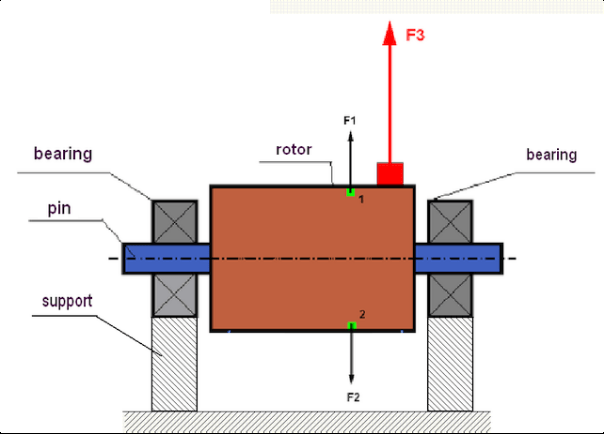
fig.1 Rotor and centrifugal forces.
In a perfectly balanced rotor, its mass is distributed symmetrically regarding the axis of the rotation. This means that any element of the rotor can correspond to another element located symmetrically in a relation to the axis of the rotation. During rotation, each rotor element acts upon by a centrifugal force directed in the radial direction (perpendicular to the axis of the rotor rotation). In a balanced rotor, the centrifugal force influencing any element of the rotor is balanced by the centrifugal force that influences the symmetrical element. For example, elements 1 and 2 (shown in fig.1 and colored in green) are influenced by centrifugal forces F1 and F2: equal in value and absolutely opposite in directions. This is true for all symmetrical elements of the rotor and thus the total centrifugal force influencing the rotor is equal to 0 the rotor is balanced. But if the symmetry of the rotor is broken (in Figure 1, the asymmetric element is marked in red), then the unbalanced centrifugal force F3 begins to act on the rotor.
When rotating, this force changes the direction together with the rotation of the rotor. The dynamic load resulting from this force is transferred to the bearings, which leads to their accelerated wear. In addition, under the influence of this variable force, there is a cyclic deformation of the supports and of the foundation on which the rotor is fixed, which produces vibration. To eliminate the imbalance of the rotor and the accompanying vibration, it is necessary to set balancing masses, that will restore the symmetry of the rotor.
Rotor balancing is an operation to eliminate imbalance by adding balancing masses.
The task of balancing is to find the value and places (angle) of the installation of one or more balancing masses.
The types of rotors and imbalance
Considering the strength of the rotor material and the magnitude of the centrifugal forces influencing it, the rotors can be divided into two types: rigid and flexible.
Rigid rotors at operating conditions under the influence of centrifugal force may get slightly deformed and the influence of this deformation in the calculations may therefore be neglected.
Deformation of flexible rotors on the other hand should never be neglected. The deformation of flexible rotors complicates the solution for the balancing problem and requires the use of some other mathematical models in comparison with the task of balancing rigid rotors. It is important to mention that the same rotor at low speeds of rotation can behave like rigid one and at high speeds it will behave like flexible one. Further on we will consider the balancing of rigid rotors only.
Depending on the distribution of imbalanced masses along the length of the rotor, two types of imbalance can be distinguished – static and dynamic. The same applies to the static and the dynamic rotor balancing.
The static imbalance of the rotor occurs without the rotation of the rotor. In other words, it is quiescent when the rotor is under the influence of gravity and in addition it turns the “heavy point” down. An example of a rotor with the static imbalance is presented in Fig.2

Fig.2
The dynamic imbalance occurs only when the rotor spins.
An example of a rotor with the dynamic imbalance is presented in Fig.3.
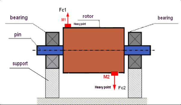
Fig.3. Dynamic imbalance of rotor – couple of the centrifugal forces
In this case, imbalanced equal masses M1 and M2 are located in different surfaces – in different places along the length of the rotor. In the static position, i.e. when the rotor does not spin, the rotor may only be influenced by gravity and the masses therefore will balance each other. In dynamics when the rotor is spinning, the masses M1 and M2 start to be influenced by centrifugal forces FЎ1 and FЎ2. These forces are equal in value and are opposite in the direction. However, since they are located in different places along the length of the shaft and are not on the same line, the forces do not compensate each other. The forces of FЎ1 and FЎ2 create a moment impacted to the rotor. That is why this imbalance has another name “momentary”. Accordingly, non-compensated centrifugal forces influence the bearing supports, which can significantly exceed the forces that we relied on and also reduce the service life for the bearings.
Since this type of imbalance occurs only in dynamics during the rotor spinning, thus it is called dynamic. It can not be eliminated in the static balancing (or so called “on the knives”) or in any other similar ways. To eliminate the dynamic imbalance, it is necessary to set two compensating weights that will create a moment equal in value and opposite in direction to the moment arising from the masses of M1 and M2. Compensating masses do not necessarily have to be installed opposite to the masses M1 and M2 and be equal to them in value. The most important thing is that they create a moment that fully compensates right at the moment of imbalance.
In general, the masses M1 and M2 may not be equal to each other, so there will be a combination of static and dynamic imbalance. It is theoretically proved that for a rigid rotor to eliminate its imbalance it is necessary and sufficient to install two weights spaced along the length of the rotor. These weights will compensate both the moment resulting from the dynamic imbalance and the centrifugal force resulting from the asymmetry of the mass relative to the rotor axis (static imbalance). As usual the dynamic imbalance is typical for long rotors, such as shafts, and static - for narrow. However, if the narrow rotor is mounted skewed in reference to the axis, or worse, deformed (the so-called "wheel wobbles"), in this case it will be difficult to eliminate the dynamic imbalance (see Fig.4), due to the fact that it is difficult to set correcting weights, that create the right compensating moment.
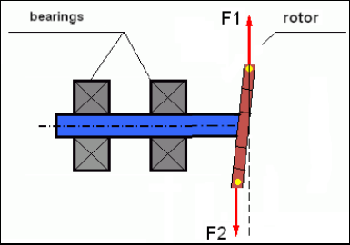
Fig.4 Dynamic balancing of the wobbling wheel
Since the narrow rotor shoulder creates a short moment, it may require correcting weights of a large mass. But at the same time there is an additional so-called “induced imbalance” associated with the deformation of the narrow rotor under the influence of centrifugal forces from the correcting masses.
See the example:
" Methodical instructions on rigid rotors balancing" ISO 1940-1:2003 Mechanical vibration – Balance quality requirements for rotors in a constant (rigid) state – Part 1: Specification and verification of balance tolerances
This is visible for narrow fan wheels, which, in addition to the power imbalance, also influences an aerodynamic imbalance. And it is important to bear in mind that the aerodynamic imbalance, in fact the aerodynamic force, is directly proportional to the angular velocity of the rotor, and to compensate it, the centrifugal force of the correcting mass is used, which is proportional to the square of the angular velocity. Therefore, the balancing effect may only occur at a specific balancing frequency. At other speeds there would be an additional gap. The same can be said about electromagnetic forces in an electromagnetic motor, which are also proportional to the angular velocity. In other words it is impossible to eliminate all causes of vibration of the mechanism by any means of balancing.
Fundamentals of Vibration
Vibration is a reaction of the mechanism design to the effect of cyclic excitation force. This force can may a different nature.
- The centrifugal force arising due to the imbalance of the rotor is an uncompensated force influencing the "heavy point". Particularly this force and also the vibration caused by it are eliminated by the rotor balancing.
- Interacting forces, that have a “geometric” nature and arise out of errors in the manufacture and installation of mating parts. These forces can occur, for instance, due to the non-roundness of the shaft journal, errors in the tooth profiles in gears, the waviness of the bearing treadmills, misalignment of the mating shafts, etc. in case of non-roundness of the necks, the shaft axis will shift depending on the angle of rotation of the shaft. Although this vibration is manifested at the rotor speed, it is almost impossible to eliminate it with the balancing.
- Aerodynamic forces arising from the rotation of the impeller fans and other blade mechanisms. Hydrodynamic forces arising from the rotation of hydraulic pump impellers, turbines, etc.
- Electromagnetic forces arising from the operation of electric machines as a result, for example, due to the asymmetry of the rotor windings, the presence of short-circuited turns, etc.
The magnitude of vibration (for example, its amplitude AB) depends not only on the magnitude of the excitation force Fт acting on the mechanism with the circular frequency ω, but also on the stiffness k of the structure of the mechanism, its mass m, and damping coefficient C.

Various types of sensors can be used to measure vibration and balance mechanisms, including:
- absolute vibration sensors designed to measure vibration acceleration (accelerometers) and vibration velocity sensors;
- relative vibration sensors eddy-current or capacitive, designed to measure vibration.
In some cases (when the structure of the mechanism allows it) sensors of force can also be used to examine its vibration weight.
Particularly, they are widely used to measure the vibration weight of the supports of hardbearing balancing machines.
Therefore vibration is the reaction of the mechanism to the influence of external forces. The amount of vibration depends not only on the magnitude of the force acting on the mechanism, but also on the rigidity of the mechanism. Two forces with the same magnitude can lead to different vibrations. In mechanisms with a rigid support structure, even with the small vibration, the bearing units can be significantly influenced by dynamic weights. Therefore, when balancing mechanisms with stiff legs apply the force sensors, and vibration (vibro accelerometers). Vibration sensors are only used on mechanisms with relatively pliable supports, right when the action of unbalanced centrifugal forces leads to a noticeable deformation of the supports and vibration. Force sensors are used in rigid supports even when significant forces arising from imbalance do not lead to significant vibration.
The resonance of the structure
We have previously mentioned that rotors are divided into rigid and flexible. The rigidity or flexibility of the rotor should not be confused with the stiffness or mobility of the supports (foundation) on which the rotor is located. The rotor is considered rigid when its deformation (bending) under the action of centrifugal forces can be neglected. The deformation of the flexible rotor is relatively large: it cannot be neglected.
In this article we only study the balancing of rigid rotors. The rigid (non-deformable) rotor in its turn can be located on rigid or movable (malleable) supports. It is clear that this stiffness/mobility of the supports is relative depending on the speed of rotation of the rotor and the magnitude of the resulting centrifugal forces. The conventional border is the frequency of free oscillations of the rotor supports/foundation. For mechanical systems, the shape and frequency of the free oscillations are determined by the mass and elasticity of the elements of the mechanical system. That is, the frequency of natural oscillations is an internal characteristic of the mechanical system and does not depend on external forces. Being deflected from the equilibrium state, supports tend to return to its equilibrium position due to the elasticity. But due to the inertia of the massive rotor, this process is in the nature of damped oscillations. These oscillations are their own oscillations of the rotor-support system. Their frequency depends on the ratio of the rotor mass and the elasticity of the supports.

When the rotor begins to rotate and the frequency of its rotation approaches the frequency of its own oscillations, the vibration amplitude increases sharply, which can even lead to the destruction of the structure.
There is a phenomenon of mechanical resonance. In the resonance region, a change in the speed of rotation by 100 rpm can lead to an increase in a vibration tenfold. In this case (in the resonance region) the vibration phase changes by 180°.
If the design of the mechanism is poorly designed, and the operating speed of the rotor is close to the natural frequency of oscillations, the operation of the mechanism becomes impossible due to unacceptably high vibration. Standard balancing methods are also impossible, as parameters change dramatically even with a slight change in the speed of rotation. Special methods in the field of resonance balancing are used but they are not well-described in this article. You can determine the frequency of natural oscillations of the mechanism on the run-out (when the rotor is turned off) or by impact with subsequent spectral analysis of the system response to the shock. The "Balanset-1" provides the ability to determine the natural frequencies of mechanical structures by these methods.
For mechanisms whose operating speed is higher than the resonance frequency, that is, operating in the resonant mode, supports are considered as mobile ones and vibration sensors are used to measure, mainly vibration accelerometers that measure the acceleration of structural elements. For mechanisms operating in hard bearing mode, supports are considered as rigid. In this case, force sensors are used.
Linear and nonlinear models of the mechanical system
Mathematical models (linear) are used for calculations when balancing rigid rotors. The linearity of the model means that one model is directly proportionally (linearly) dependent on the other. For example, if the uncompensated mass on the rotor is doubled, then the vibration value will be doubled correspondingly. For rigid rotors you can use a linear model because such rotors are not deformed. It is no longer possible to use a linear model for flexible rotors. For a flexible rotor, with an increase of the mass of a heavy point during rotation, an additional deformation will occur, and in addition to the mass, the radius of the heavy point will also increase. Therefore, for a flexible rotor, the vibration will more than double, and the usual calculation methods will not work. Also, a violation of the linearity of the model can lead to a change in the elasticity of the supports at their large deformations, for example, when small deformations of the supports work some structural elements, and when large in the work include other structural elements. Therefore it is impossible to balance the mechanisms that are not fixed at the base, and, for example, are simply established on a floor. With significant vibrations, the unbalance force can detach the mechanism from the floor, thereby significantly changing the stiffness characteristics of the system. The engine legs must be securely fastened, bolted fasteners tightened, the thickness of the washers must provide sufficient rigidity, etc. With broken bearings, a significant displacement of the shaft and its impacts is possible, which will also lead to a violation of linearity and the impossibility of carrying out high-quality balancing.
Methods and devices for balancing
As mentioned above, balancing is the process of combining the main Central axis of inertia with the axis of rotation of the rotor.
The specified process can be executed in two ways.
The first method involves the processing of the rotor axles, which is performed in such a way that the axis passing through the centers of the section of the axles with the main Central axis of inertia of the rotor. This technique is rarely used in practice and will not be discussed in detail in this article.
The second (most common) method involves moving, installing or removing corrective masses on the rotor, which are placed in such a way that the axis of inertia of the rotor is as close as possible to the axis of its rotation.
Moving, adding or removing corrective masses during balancing can be done using a variety of technological operations, including: drilling, milling, surfacing, welding, screwing or unscrewing screws, burning with a laser beam or electron beam, electrolysis, electromagnetic welding, etc.
The balancing process can be performed in two ways:
- balanced rotors Assembly (in its own bearings);
- balancing of rotors on balancing machines.
To balance the rotors in their own bearings we usually use specialized balancing devices (kits), which allows us to measure the vibration of the balanced rotor at the speed of its rotation in a vector form, i.e. to measure both the amplitude and phase of vibration.
Currently, these devices are manufactured on the basis of microprocessor technology and (in addition to the measurement and analysis of vibration) provide automated calculation of the parameters of corrective weights that must be installed on the rotor to compensate its imbalance.
These devices include:
- – measuring and computing unit, made on the basis of a computer or industrial controller;
- two (or more) vibration sensors;
- phase angle sensor;
- equipment for installation of sensors at the facility;
- specialized software designed to perform a full cycle of measurement of rotor unbalance parameters in one, two or more planes of correction.
For balancing rotors on balancing machines in addition to a specialized balancing device (measuring system of the machine) it is required to have an “unwinding mechanism” designed to install the rotor on the supports and ensure its rotation at a fixed speed.
Currently, the most common balancing machines exist in two types:
- over-resonant (with supple supports);
- hard bearing (with rigid supports).
Over-resonant machines have a relatively pliable supports, made, for example, on the basis of the flat springs.
The natural oscillation frequency of these supports is usually 2-3 times lower than the speed of the balanced rotor, which is mounted on them.
Vibration sensors (accelerometers, vibration velocity sensors, etc.) are usually used to measure the vibration of the supports of a resonant machine.
In the hardbearing balancing machines are used relatively-rigid supports, natural oscillation frequencies of which should be 2-3 times higher than the speed of the balanced rotor.
Force sensors are usually used to measure the vibration weight on the supports of the machine.
The advantage of the hard bearing balancing machines is that they can be balanced at relatively low rotor speeds (up to 400-500 rpm), which greatly simplifies the design of the machine and its foundation, as well as increases the productivity and safety of balancing.
Balancing technique
Balancing eliminates only the vibration which is caused by the asymmetry of the rotor mass distribution relative to its axis of rotation. Other types of the vibration cannot be eliminated by the balancing!
Balancing is the subject to technically serviceable mechanisms, the design of which ensures the absence of resonances at the operating speed, securely fixed on the foundation, installed in serviceable bearings.
The faulty mechanism is the subject to a repair, and only then – to a balancing. Otherwise, qualitative balancing impossible.
Balancing cannot be a substitute for repair!
The main task of balancing is to find the mass and the place (angle) of installation of compensating weights, which are balanced by centrifugal forces.
As mentioned above, for rigid rotors it is generally necessary and sufficient to install two compensating weights. This will eliminate both the static and dynamic rotor imbalance. A general scheme of the vibration measurement during balancing looks like the following:
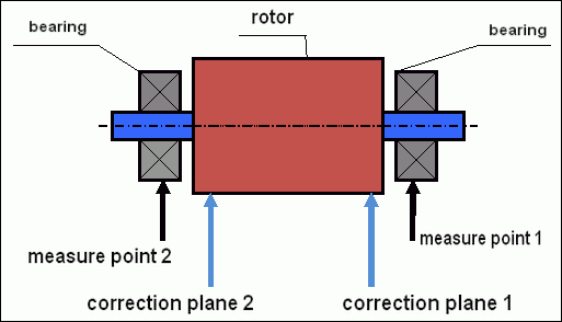
fig.5 Dynamic balancing – correction planes and measure points
Vibration sensors are installed on the bearing supports at points 1 and 2. The speed mark is fixed right on the rotor, a reflective tape is glued usually. The speed mark is used by the laser tachometer to determine the speed of the rotor and the phase of the vibration signal.
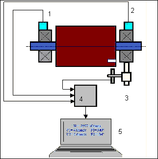
fig. 6. Installation of sensors during balancing in two planes, using Balanset-1
1,2-vibration sensors, 3-phase, 4- USB measuring unit, 5-laptop
In most cases, dynamic balancing is carried out by the method of three starts. This method is based on the fact that test weights of an already-known mass are installed on the rotor in series in 1 and 2 planes; so the masses and the place of installation of balancing weights are calculated based on the results of changing the vibration parameters.
The place of installation of the weight is called the correction plane. Usually, the correction planes are selected in the area of the bearing supports on which the rotor is mounted.
The initial vibration is measured at the first start. Then, a trial weight of a known mass is installed on the rotor closer to one of the supports. Then the second start is performed, and we measure the vibration parameters, that should change because of the installation of the trial weight. Then the trial weight in the first plane is removed and installed in the second plane. The third start-up is performed and the vibration parameters are measured. When the trial weight is removed, the program automatically calculates the mass and the place (angles) of the installation of balancing weights.
ಅಸಮತೋಲನ ಬದಲಾವಣೆಗೆ ಸಿಸ್ಟಮ್ ಹೇಗೆ ಪ್ರತಿಕ್ರಿಯಿಸುತ್ತದೆ ಎಂಬುದನ್ನು ನಿರ್ಧರಿಸುವುದು ಪರೀಕ್ಷಾ ತೂಕವನ್ನು ಹೊಂದಿಸುವ ಅಂಶವಾಗಿದೆ. ನಾವು ದ್ರವ್ಯರಾಶಿಗಳು ಮತ್ತು ಮಾದರಿ ತೂಕದ ಸ್ಥಳವನ್ನು ತಿಳಿದಾಗ, ಪ್ರೋಗ್ರಾಂ ಪ್ರಭಾವದ ಗುಣಾಂಕಗಳೆಂದು ಕರೆಯಲ್ಪಡುವದನ್ನು ಲೆಕ್ಕಾಚಾರ ಮಾಡಬಹುದು, ತಿಳಿದಿರುವ ಅಸಮತೋಲನದ ಪರಿಚಯವು ಕಂಪನ ನಿಯತಾಂಕಗಳ ಮೇಲೆ ಹೇಗೆ ಪರಿಣಾಮ ಬೀರುತ್ತದೆ ಎಂಬುದನ್ನು ತೋರಿಸುತ್ತದೆ. ಪ್ರಭಾವದ ಗುಣಾಂಕಗಳು ಯಾಂತ್ರಿಕ ವ್ಯವಸ್ಥೆಯ ಗುಣಲಕ್ಷಣಗಳಾಗಿವೆ ಮತ್ತು ಬೆಂಬಲಗಳ ಬಿಗಿತ ಮತ್ತು ರೋಟರ್-ಬೆಂಬಲ ವ್ಯವಸ್ಥೆಯ ದ್ರವ್ಯರಾಶಿಯನ್ನು (ಜಡತ್ವ) ಅವಲಂಬಿಸಿರುತ್ತದೆ.
ಅದೇ ವಿನ್ಯಾಸದ ಒಂದೇ ರೀತಿಯ ಕಾರ್ಯವಿಧಾನಗಳಿಗೆ, ಪ್ರಭಾವದ ಗುಣಾಂಕಗಳು ಹೋಲುತ್ತವೆ. ನೀವು ಅವುಗಳನ್ನು ನಿಮ್ಮ ಕಂಪ್ಯೂಟರ್ ಮೆಮೊರಿಯಲ್ಲಿ ಉಳಿಸಬಹುದು ಮತ್ತು ಪರೀಕ್ಷಾ ರನ್ಗಳನ್ನು ನಡೆಸದೆ ಅದೇ ರೀತಿಯ ಕಾರ್ಯವಿಧಾನಗಳನ್ನು ಸಮತೋಲನಗೊಳಿಸಲು ನಂತರ ಅವುಗಳನ್ನು ಬಳಸಬಹುದು, ಇದು ಸಮತೋಲನದ ಕಾರ್ಯಕ್ಷಮತೆಯನ್ನು ಹೆಚ್ಚು ಸುಧಾರಿಸುತ್ತದೆ. ಪರೀಕ್ಷಾ ತೂಕವನ್ನು ಸ್ಥಾಪಿಸುವಾಗ ಕಂಪನ ನಿಯತಾಂಕಗಳು ಗಮನಾರ್ಹವಾಗಿ ಬದಲಾಗುವಂತೆ ಪರೀಕ್ಷಾ ತೂಕದ ದ್ರವ್ಯರಾಶಿಯನ್ನು ಆಯ್ಕೆ ಮಾಡಬೇಕು ಎಂದು ನಾವು ಗಮನಿಸಬೇಕು. ಇಲ್ಲದಿದ್ದರೆ, ಪರಿಣಾಮದ ಗುಣಾಂಕಗಳನ್ನು ಲೆಕ್ಕಾಚಾರ ಮಾಡುವ ದೋಷವು ಹೆಚ್ಚಾಗುತ್ತದೆ ಮತ್ತು ಸಮತೋಲನದ ಗುಣಮಟ್ಟವು ಹದಗೆಡುತ್ತದೆ.
A guide to the device Balanset-1 provides a formula by which you can approximately determine the mass of the trial weight, depending on the mass and the speed of the rotation of the balanced rotor. As you can understand from Fig. 1 the centrifugal force acts in the radial direction, i.e. perpendicular to the rotor axis. Therefore, vibration sensors should be installed so that their sensitivity axis is also directed in the radial direction. Usually the rigidity of the foundation in the horizontal direction is less, so the vibration in the horizontal direction is higher. Therefore, to increase the sensitivity of the sensors should be installed so that their axis of sensitivity could also be directed horizontally. Although there is no fundamental difference. In addition to the vibration in the radial direction, it is necessary to control the vibration in the axial direction, along the axis of rotation of the rotor. This vibration is usually caused not by imbalance, but by other reasons, mainly due to misalignment and misalignment of shafts connected through the coupling. This vibration is not eliminated by balancing, in this case alignment is required. In practice, usually in such mechanisms there is an imbalance of the rotor and misalignment of the shafts, which greatly complicates the task of eliminating the vibration. In such cases, you must first align and then balance the mechanism. (Although with a strong torque imbalance, vibration also occurs in the axial direction due to the" twisting " of the foundation structure).
Measurement Accuracy and Error Analysis
Understanding measurement accuracy is critical for professional balancing operations. The Balanset-1A provides the following measurement precision:
| ಪ್ಯಾರಾಮೀಟರ್ | Accuracy Formula | Example (for typical values) |
|---|---|---|
| RMS Vibration Velocity | ±(0.1 + 0.1×Vಅಳೆಯಲಾದ) mm/sec | For 5 mm/sec: ±0.6 mm/sec For 10 mm/sec: ±1.1 mm/sec |
| Rotation Frequency | ±(1 + 0.005×Nಅಳೆಯಲಾದ) rpm | For 1000 rpm: ±6 rpm For 3000 rpm: ±16 rpm |
| ಫೇಜ್ ಮಾಪನ | ±1° | Constant accuracy across all speeds |
⚠️ Critical for Accurate Balancing
- !Trial weight must cause >20-30% amplitude change and/or >20-30° phase change
- !If changes are smaller, measurement errors significantly increase
- !Vibration amplitude and phase stability should not vary more than 10-15% between measurements
- !If variation exceeds 15%, check for resonance conditions or mechanical issues
Criteria for assessing the quality of balancing mechanisms
ರೋಟರ್ (ಮೆಕ್ಯಾನಿಸಂ) ಸಮತೋಲನದ ಗುಣಮಟ್ಟವನ್ನು ಎರಡು ರೀತಿಯಲ್ಲಿ ಅಂದಾಜು ಮಾಡಬಹುದು. ಮೊದಲ ವಿಧಾನವು ಸಮತೋಲನದ ಸಮಯದಲ್ಲಿ ನಿರ್ಧರಿಸಲಾದ ಉಳಿದ ಅಸಮತೋಲನದ ಮೌಲ್ಯವನ್ನು ಉಳಿದ ಅಸಮತೋಲನದ ಸಹಿಷ್ಣುತೆಯೊಂದಿಗೆ ಹೋಲಿಸುವುದನ್ನು ಒಳಗೊಂಡಿರುತ್ತದೆ. ಸ್ಟ್ಯಾಂಡರ್ಡ್ನಲ್ಲಿ ಸ್ಥಾಪಿಸಲಾದ ವಿವಿಧ ವರ್ಗಗಳ ರೋಟರ್ಗಳಿಗೆ ನಿರ್ದಿಷ್ಟಪಡಿಸಿದ ಸಹಿಷ್ಣುತೆಗಳು ISO 21940-11 «Mechanical vibration – Rotor balancing – Part 11: Procedures and tolerances for rotors with rigid behaviour» (formerly ISO 1940-1).
However, the implementation of these tolerances can not fully guarantee the operational reliability of the mechanism associated with the achievement of a minimum level of vibration. This is due to the fact that the vibration of the mechanism is determined not only by the amount of force associated with the residual imbalance of its rotor, but also depends on a number of other parameters, including: the rigidity K of the structural elements of the mechanism, its mass M, damping coefficient, and the speed. Therefore, to assess the dynamic qualities of the mechanism (including the quality of its balance) in some cases, it is recommended to assess the level of residual vibration of the mechanism, which is regulated by a number of standards.
ಯಾಂತ್ರಿಕತೆಗಳ ಅನುಮತಿಸುವ ಕಂಪನ ಮಟ್ಟವನ್ನು ನಿಯಂತ್ರಿಸುವ ಅತ್ಯಂತ ಸಾಮಾನ್ಯ ಮಾನದಂಡವಾಗಿದೆ ISO 10816-3:2009 Preview Mechanical vibration — Evaluation of machine vibration by measurements on non-rotating parts — Part 3: Industrial machines with nominal power above 15 kW and nominal speeds between 120 r/min and 15 000 r/min when measured in situ.»
ಅದರ ಸಹಾಯದಿಂದ, ನೀವು ಎಲ್ಲಾ ರೀತಿಯ ಯಂತ್ರಗಳಲ್ಲಿ ಸಹಿಷ್ಣುತೆಯನ್ನು ಹೊಂದಿಸಬಹುದು, ಅವುಗಳ ವಿದ್ಯುತ್ ಡ್ರೈವ್ನ ಶಕ್ತಿಯನ್ನು ಗಣನೆಗೆ ತೆಗೆದುಕೊಳ್ಳಲಾಗುತ್ತದೆ.
ಈ ಸಾರ್ವತ್ರಿಕ ಮಾನದಂಡದ ಜೊತೆಗೆ, ನಿರ್ದಿಷ್ಟ ರೀತಿಯ ಕಾರ್ಯವಿಧಾನಗಳಿಗಾಗಿ ಅಭಿವೃದ್ಧಿಪಡಿಸಲಾದ ಹಲವಾರು ವಿಶೇಷ ಮಾನದಂಡಗಳಿವೆ. ಉದಾಹರಣೆಗೆ,
- ISO 14694:2003 "Industrial fans – Specifications for balance quality and vibration levels"
- ISO 7919-1-2002 “Vibration of machines without reciprocating motion. Measurements on rotating shafts and evaluation criteria. General guidance.»
🛡️ Important Safety Considerations for EU Compliance
- !Risk Assessment Required: Perform EN ISO 12100 risk assessment before balancing operations
- !Qualified Personnel: Only trained and certified personnel should perform balancing operations
- !Personal Protective Equipment: Always use appropriate PPE per EN 166 (eye protection) and EN 352 (hearing protection)
- !Emergency Procedures: Establish clear emergency shutdown procedures and ensure all operators are familiar with them
- !ದಾಖಲೆಗಳು: Maintain detailed records of all balancing operations for traceability and compliance
EU Compliance and Safety Information
ಅನುಸರಣೆ ಘೋಷಣೆ
The Balanset-1A portable balancer complies with the following European Union directives and standards:
| EU Directive/Standard | Compliance Details | Safety Requirements |
|---|---|---|
| Machinery Directive 2006/42/EC | Safety requirements for machinery and safety components | Risk assessment, safety instructions, CE marking |
| EMC Directive 2014/30/EU | Electromagnetic compatibility requirements | Immunity to electromagnetic interference |
| RoHS Directive 2011/65/EU | Restriction of hazardous substances | Lead-free, mercury-free, cadmium-free components |
| WEEE Directive 2012/19/EU | Waste electrical and electronic equipment | Proper disposal and recycling procedures |
| EN ISO 12100:2010 | Safety of machinery - General principles for design | Risk assessment and risk reduction |
| EN 60825-1:2014 | Safety of laser products - Part 1 | Class 2 laser safety requirements |
| EN ISO 14120:2015 | Guards - General requirements | Protection against rotating machinery hazards |
Electrical Safety Standards
- ✓EN 61010-1: Safety requirements for electrical equipment for measurement, control, and laboratory use
- ✓EN 60950-1: Information technology equipment safety (USB powered device)
- ✓IEC 61000 series: Electromagnetic compatibility standards
- ✓Operating voltage: 5V DC via USB (Extra Low Voltage)
- ✓Power consumption: < 2.5W
- ✓Protection class: IP54 (dust-protected; splash-water resistant)
Rotating Equipment Safety
⚠️ Mandatory Safety Procedures (EN ISO 12100)
WARNING: When working with rotating machinery, observe the following safety requirements:
- !EN ISO 14118: Prevention of unexpected start-up - Use lockout/tagout procedures before sensor installation
- !EN ISO 14120: Ensure all rotating equipment is properly guarded
- !EN ISO 13857: Maintain minimum safe distances from rotating parts (500mm for body, 120mm for fingers)
- !Personal Protective Equipment: Wear safety glasses per EN 166, hearing protection per EN 352, and avoid loose clothing
- !Never install sensors or trial weights on rotating machinery while in motion
- !Ensure machine is completely stopped and secured before sensor installation
- !জরুরী ನಿಲುಗಡೆ: Must be accessible within 3 meters of operator position
- !Only qualified and certified personnel should perform balancing operations
Laser Safety Classification
🔴 Class 2 Laser Device (EN 60825-1:2014)
- Wavelength: 650 nm (Red visible light)
- Maximum output power: < 1 mW
- Beam diameter: 3-5 mm at 100mm distance
- Divergence: < 1.5 mrad
- Safety classification: Eye safe for momentary exposure (< 0.25 sec)
- Required labeling: "LASER RADIATION - DO NOT STARE INTO BEAM - CLASS 2 LASER PRODUCT"
- Access class: Unrestricted (general access permitted)
Laser Safety Procedures:
- Never intentionally stare into laser beam
- Do not aim laser at persons, vehicles, or aircraft
- Avoid viewing laser beam with optical instruments (telescopes, binoculars)
- Be aware of specular reflections from shiny surfaces
- Turn off laser when not in use
- Report any eye exposure incidents immediately
- Use laser safety glasses (OD 2+ at 650nm) for extended exposure
Measurement Accuracy and Calibration
| ಪ್ಯಾರಾಮೀಟರ್ | ನಿಖರತೆ | Calibration Frequency |
|---|---|---|
| ಕಂಪನ ವೈಶಾಲ್ಯ | ಓದಿನ ±5% | Annually or after 1000 hours |
| Phase measurement | ±1° | Annually |
| Rotation speed | ±0.1% of reading | Annually |
| Sensor sensitivity | 13 mV/(mm/s) ±10% | When replacing sensors |
Environmental Compliance
- ✓Operating environment: 5°C to 50°C, < 85% RH non-condensing
- ✓Storage environment: -20°C to 70°C, < 95% RH non-condensing
- ✓Altitude: Up to 2000m above sea level
- ✓Vibration resistance: IEC 60068-2-6 (10-500 Hz, 2g acceleration)
- ✓ಆಘಾತ ನಿರೋಧಕತೆ: IEC 60068-2-27 (15g, 11ms duration)
- ✓IP rating: IP54 (dust-protected; splash-water resistant)
Operation Requirements
- ✓Operators must be trained in machinery safety per EU standards
- ✓Risk assessment required per EN ISO 12100 before use
- ✓Maintain equipment per manufacturer specifications
- ✓Report any safety incidents or equipment malfunctions immediately
- ✓Maintain detailed records of all balancing operations for traceability
ದಾಖಲೀಕರಣದ ಅವಶ್ಯಕತೆಗಳು
For EU compliance, maintain the following documentation:
- ✓Risk assessment documentation per EN ISO 12100
- ✓Operator training records and certifications
- ✓Equipment calibration and maintenance logs
- ✓Balancing operation records with dates, operators, and results
- ✓Safety incident reports and corrective actions
- ✓Equipment modification or repair documentation
Technical Support and Service
For technical support, calibration services, and spare parts:
- ✓Manufacturer: ವೈಬ್ರೊಮೆರಾ
- ✓ಸ್ಥಳ: Narva, Estonia (EU)
- ✓Website: https://vibromera.eu
- ✓Support languages: All major languages. Text-based communication available.
- ✓Service coverage: Worldwide shipping available
- ✓ವಾರಂಟಿ: 12 months from date of purchase
- ✓Calibration service: Available through authorized service centers