Avto-spektrni tushunish


The auto-spectrum — autospektrum deb ham yoziladi, quvvat spektri yoki shunchaki “spektr” deb ham ataladi — bitta signalning chastota sohasidagi vibration signal, ushbu signal’ning energiyasi yoki amplitude chastotalar bo'yicha qanday taqsimlanishini ko'rsatadi. U vaqt yozuvining Tez Furye o'zgarishi (FFT) ni olib, har bir chastota komponentining amplitudasini ko'rsatish yo'li bilan hosil qilinadi. “Avto-” prefiksi uni cross-spectrum, ikki xil signalni bog'laydigan funksiyadan farqlaydi: avto-spektr — signalning o'zi bilan olingan spektridir.
Kundalik amaliyotda texnikchilarning aksariyati “spektr” yoki “FFT” deganda aynan shuni nazarda tutadi — har qanday tebranish analizatoridagi standart chastota ko'rinishi, uning cho'qqilari unbalance, podshipnik nosozlik chastotalariga, gear meshva boshqalarda. Bu kundalik vosita texnik jihatdan avto-spektr ekanligini anglash, ko'p kanalli ishga o'tganda ayniqsa muhim bo'lib qoladi — u yerda o'zaro spektrlar, coherenceva boshqa korrelyatsiya funksiyalari ishga kiradi.
1. Matematik asos
Bir xil natijaga erishishning ikki yo'li
Avto-spektrga erishishning matematik jihatdan teng ikkita yo'li mavjud:
- Direct FFT: vaqt signalini o'zgartiring, har bir murakkab FFT katakchasining amplitudasini (yoki amplituda kvadratini) oling va uni chastotaga nisbatan grafik ko'rinishida tasvirlang. Bu deyarli har qanday o'lchov asbobida qo'llaniladigan oddiy va keng tarqalgan usuldir.
- Avtokorrelatsiya orqali: avval signalning avtokorrelyatsiya funksiyasini hisoblang, so’ngra uning FFT sini oling. Shunga ko’ra Viner–Xinchen teoremasi natija to’g’ridan-to’g’ri usul bilan bir xil bo’ladi — boshqa hisoblash yo’li orqali olingan xuddi shu spektr.
Magnitud kvadratga oshirilsa va birlik chastotaga normallashtirilsa, xuddi shu miqdor quvvat spektral zichligiga aylanadi, bu keng polosali tasodifiy tebranishlar uchun afzal ko’rilgan shakl hisoblanadi.
Barqarorlik uchun o’rtacha qiymat olish
Bitta FFT statistik jihatdan shovqinli bo’ladi, shuning uchun ketma-ket vaqt yozuvlaridan hisoblangan bir nechta avto-spektr o’rtachalanadi — bu taxminni barqarorlashtiradi va tasodifiy tarqalishni kamaytiradi. Odatiy mashina diagnostikasi uchun 4–16 ta o’rtacha qiymat tipik hisoblanadi; keng polosali tasodifiy tebranishlar uchun 50–100 yoki undan ko’proq o’rtacha qiymat talab qilinishi mumkin. Bundan kelgan foyda o’lchov vaqti hisobiga erishiladi, shuning uchun o’rtacha qiymatlar soni “ko’proq doimo yaxshiroq” emas, balki ataylab qilingan murosaga asoslanadi.
2. Aniqlovchi xususiyatlar
Har qanday spektrni o’qiyotganda yodda tutishga arziydigang uchta xususiyat matematikadan bevosita kelib chiqadi:
- Real-valued: avto-spektrda mavhum qism yo’q. U faqat amplitudani ifodalaydi, shuning uchun phase asl signalning fazasi magnitud hisobida yo’qoladi. Bir nuqtali nosozliklarni aniqlash uchun bu yo’qotish emas; ammo balanslashtirish yoki o’tkazish funksiyasini hisoblashda, faza muhim bo’lgan holatlarda, bu haqiqiy cheklovdir.
- Har doim musbat: qiymatlar har doim noldan katta yoki teng bo’ladi, chunki ular energiya yoki quvvatni ifodalaydi va bu salbiy bo’lishi mumkin emas.
- Haqiqiy signallar uchun simmetrik: haqiqiy vaqt signalining spektri Nyukvist chastotasi atrofida simmetrik bo’ladi — manfiy chastotalar shunchaki musbatlarni aks ettiradi — shuning uchun faqat musbat yarmi ko’rsatiladi va u barcha ma’lumotni o’z ichiga oladi.
3. Mashina diagnostikasida avto-spektr
Tahlilchining kundalik ko’rsatgichi
Bu texniklar doimiy ishlatiydigan grafik. U barcha tebranish chastota komponentlarini bir vaqtda ko’rsatadi va tahlilchining vazifasi har bir cho’qqini aniqlab, uni nosozlik turiga moslashtirish — bu avto-spektrni nosozliklarni tashxislash va muntazam texnik holat baholash uchun.
E'tibor Berish Kerak Bo'lgan Xususiyatlar
- 1× peak: running-speed tebranish, asosan muvozanatsizlik va boshqa aylanish davriga mos keladigan manbalar bilan belgilanadi.
- 2× peak: commonly misalignment or mexanik bo'shashish.
- Podshipnik chastotalari: BPFO, BPFI, BSF, and FTF, ko'pincha o'ralgan sidebands.
- Gear mesh: tish ilashish chastotasi va uning harmonics.
- Electrical: chiziq chastotasining ikki baravari (60 Hz ta'minotda 120 Hz, 50 Hz ta'minotda 100 Hz).
- Noise floor: tasodifiy tebranish va asbob shovqini tomonidan belgilanadigan fon darajasi, bunga nisbatan haqiqiy cho'qqilar ajralib turishi kerak.
4. Avto-Spektr va O'zaro Spektr
Bir kanalli avto-spektr “qanday chastotalar mavjud?” degan savolga javob beradi, ikki kanalli muqobili esa “ikki signal qanday bog'liq?” degan savolga javob beradi. Bu farqni aniq ko'rsatish foydalidir:
| Avto-Spektr (bir kanal) | O'zaro Spektr (ikki kanal) |
|---|---|
| Bitta signal spektri | Ikki signal o'rtasidagi bog'liqlik |
| Ushbu signalning chastota tarkibini ko'rsatadi | Ikkalasiga xos umumiy chastota tarkibini ko'rsatadi |
| Faza ma'lumoti yo'q | Faza bog'liqligini o'z ichiga oladi |
| Ko'pchilik diagnostika uchun yetarli | Underpins o'tkazish funksiyasi va kogerentlik tahlili |
| Standart bir kanalli FFT | Ikki sinxronlashtirilgan kanal talab etiladi |
5. O'rtalashtirish rejimlari va ko'rsatish imkoniyatlari
O'rtalashtirish rejimini tanlash
- Chiziqli o'rtalashtirish: ketma-ket spektrlarning oddiy arifmetik o'rtachasi bo'lib, tasodifiy shovqinni kamaytiradi va haqiqiy spektrga yaqinlashadi — mexanizm tahlili uchun standart usul.
- Eksponensial o'rtalashtirish: eng so'nggi yozuvlarga ustunlik beradigan og'irlikli o'rtacha; sharoitlar o'zgarib turadigan real vaqtli monitoring uchun eng maqbul.
- Cho'qqi qiymatni ushlab qolish (maksimal spektr): har bir chastota katagida qayd etilgan eng yuqori qiymat saqlanib qoladi, o'tkinchi komponentlar aniqlanadi — buning qiymati run-up and coastdown testing.
O'qlar masshtabini sozlash
Amplituda o'qi quyidagi ko'rinishda ifodalanishi mumkin: linear scale (mm/s, m/s²), bu mutlaq qiymatlarni o'qishni osonlashtiradi, ammo katta cho'qqilar yonida kichik cho'qqilar ko'rinmasligi mumkin; yoki logarifmik dB shkalasi (20·log[amplitude/reference]), which compresses a wide dynamic range shunda kichik va katta cho'qqilar bir vaqtda ko'rinadi — batafsil va ilmiy ishlar uchun afzal ko'rilgan ko'rinish. Chastota o'qi odatda linear mexanizmlar uchun Hz da ifodalanadi, ammo logarithmic teng oktava oraliqli o'q juda keng chastota diapazonlari uchun qulay.
6. Sifat va xatolar
Spektr sifati uning asosidagi ma'lumotlar sifatiga bog'liq. A clean spectrum past shovqin fonidan aniq cho'qqilarni ko'rsatadi; a noisy spectrum yuqori fon shovqinida cho'qqilarni ko'mib qo'yadi, buni ko'proq o'rtalashtirish va yetarli chastota yechimi bartaraf etishi mumkin. Ikki ta'minlash tekshiruvi muhim: chastota yechimi yaqin joylashgan cho'qqilarni ajratish uchun yetarli darajada aniq ekanligini tasdiqlang va input overload, bu signalni qirqib tashlaydi va soxta spektral komponentlarni hosil qiladi — bu sodir bo'lsa, kirish kuchaytirishini kamaytiring va qayta yig'ing. The FFT ajratish qobiliyati kalkulyatori qiziqtirgan cho'qqilarni aniqlaydigan chiziq soni va o'tkazish polosasini tanlashga yordam beradi.
Dala asboblari qayerda qo'llaniladi
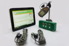
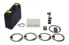
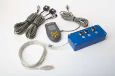
Balanset kabi ko'chma ikki kanalli qurilmada Balanset-1A, avto-spektr — bu texnik xodim energiya 1× chastotada to'plangan-qo'planganligi (muvozanatsizlikni ko'rsatib, uchun nomzod bo'lishi mumkin) yoki butunlay boshqa nosozlikni bildiruvchi podshipnik va tishli g'ildirak chastotalari bo'ylab tarqalgan-tarqalmaganligini aniqlash uchun mashina yonida o'qiydigan kundalik diagnostika ko'rinishidir. field balancing) — barchasi mashina ishlaydigan tezlikda o'z podshipniklarida qayd etiladi.
Avto-spektr tebranish diagnostikasining asosiy chastota tahlili vositasidir: texnik xodimlar nosozliklarni aniqlash va holat baholash uchun har kuni foydalanadigan bir kanalli FFT. “Spektr” texnik jihatdan avto-spektr ekanligini — va u o'zaro spektrlar va boshqa spektral funksiyalar bilan qanday bog'liqligini — tushunish ko'p kanalli tahlil va mashina diagnostikasini chuqurlashtirish uchun poydevor yaratadi.
