Understanding Synchronous Averaging

Devices

Portable balancer & Vibration analyzer Balanset-1A

€1,975.00 + VAT (if applicable)

Parts

Vibration sensor

€90.00 + VAT (if applicable)

Parts

Optical Sensor (Laser Tachometer)

€124.00 + VAT (if applicable)

Devices

Balanset-4

€6,803.00 + VAT (if applicable)

Parts

Magnetic Stand Insize-60-kgf

€46.00 + VAT (if applicable)

Parts

Reflective tape

€10.00 + VAT (if applicable)

Devices

Dynamic balancer “Balanset-1A” OEM

€1,735.00 + VAT (if applicable)

Synchronous averaging — also called time-domain averaging or time-synchronous averaging (TSA) — is a signal-processing technique in vibration analysis that enhances periodic, speed-synchronous vibration while suppressing random noise and any vibration that is not locked to shaft rotation. The method repeatedly samples the vibration over many shaft revolutions, each block triggered by a once-per-revolution tachometer pulse, then averages the corresponding points across every revolution. Components that repeat identically each turn reinforce one another, while random noise and asynchronous components cancel, producing a dramatic improvement in signal-to-noise ratio. It is especially powerful for gear diagnostics — isolating a single gear’s mesh signature — and can reveal subtle periodic patterns buried in noise that would be completely invisible in an ordinary time waveform or FFT spectrum.

1. How Synchronous Averaging Works

The process, step by step

1. Trigger signal: a once-per-revolution pulse from a tachometer or keyphasor defines the start of each revolution.
2. Data segmentation: the vibration signal is divided into equal-length segments, one per revolution.
3. Alignment: every segment is aligned to its trigger pulse so they share a common angular starting point.
4. Point-by-point averaging: corresponding samples across all segments are averaged together.
5. Result: a single averaged waveform representing one idealised revolution.
6. Noise reduction: random components cancel statistically while the periodic ones reinforce.

The mathematics behind it

• Periodic, phase-locked signals sum coherently (they add in phase, growing linearly with the number of averages).
• Random noise sums incoherently (it cancels statistically, growing only with the square root of the count).
• The signal-to-noise improvement is therefore proportional to √N, where N is the number of averages.
• For example, 100 averages improve the SNR by a factor of 10 (20 dB); 400 averages by 20× (26 dB).

Because the trigger comes from the shaft itself, synchronous averaging is inherently a form of order analysis — the averaged record is locked to shaft angle, not to clock time, so it tolerates the small speed drift that would smear an ordinary fixed-sample-rate FFT.

2. Applications

Gearbox diagnostics — the flagship use

This is the most common and most powerful application.

• Gear mesh isolation: averaging synchronously with the gear of interest enhances that gear’s mesh pattern while suppressing other gears and the bearings, helping confirm gear defects.
• Tooth-by-tooth analysis: the averaged waveform shows each tooth engagement clearly, a damaged tooth appears as a localised deviation in the otherwise repeating pattern, and the deviation lets you identify which tooth is damaged and gauge its severity.

Other applications

• Bearing analysis enhancement: averaging over an outer-race period isolates and enhances the periodic impacts of a bearing defect, cutting through the masking of other sources — particularly useful in high-noise environments.
• Torsional vibration: enhances the components synchronous with rotation while suppressing lateral vibration and noise, revealing torsional resonances and excitation.
• Balancing: improves the accuracy of amplitude and phase measurement in noisy conditions, giving more reliable influence coefficient determination.

3. Advantages

• Noise reduction: a dramatic improvement in signal-to-noise ratio that can extract signals buried 20–30 dB below the noise floor, making measurements possible in genuinely harsh environments.
• Fault isolation: separates one component’s signature from all the others — for instance isolating the pinion mesh from the gear mesh in a gearbox — and so identifies which component is defective.
• Enhanced resolution: reveals subtle patterns and defects, shows detail masked in the raw signal, and enables genuinely early fault detection.

4. Requirements and Limitations

What it requires

• Tachometer: a reliable once-per-revolution trigger is essential — without it the method cannot align the segments.
• Constant speed: speed must hold reasonably steady, typically within ±1–2%.
• Sufficient averages: usually 50–200 revolutions for a good result.
• Periodic signal: only truly periodic, phase-locked components are enhanced.

Where it falls short

• It suppresses non-synchronous faults: random defects and most bearing fault frequencies are reduced, so the technique is the wrong tool if those are what you are hunting (use envelope analysis instead).
• Speed variation: a changing speed during the averaging window blurs the result.
• Time required: data must be collected over many revolutions.
• Not real-time: some post-processing is required.

5. Comparison with Other Techniques

Synchronous averaging vs linear averaging

• Synchronous: averages in the time domain, locked to rotation, and enhances periodic components.
• Linear: averages FFT spectra and reduces random variation across all frequencies indiscriminately.
• Use cases: synchronous for gears and specific components; linear for general spectrum smoothing.

Synchronous averaging vs envelope analysis

• Synchronous averaging: time domain, enhances periodic patterns.
• Envelope analysis: frequency domain, detects repetitive impacts such as those from a spalled raceway.
• Complementary: the two can be combined for comprehensive analysis — average out the gear mesh, then envelope what remains to find a bearing defect.

6. Practical Implementation

Setup, collection and interpretation

• Setup: install a tachometer with a clear once-per-revolution pulse — a strip of reflective tape with an optical pickup is the usual field choice — set the number of averages (50–200), define the signal length (one revolution, ten revolutions, etc.), and verify speed stability.
• Data collection: acquire data over the averaging period; the instrument automatically segments and averages, displays the averaged waveform, and will often compute the FFT of that averaged signal to give an enhanced spectrum.
• Interpretation: examine the averaged waveform for periodic patterns, look for deviations that indicate defects, compare against known-good baseline signatures, and quantify severity from the deviation amplitude.

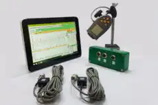
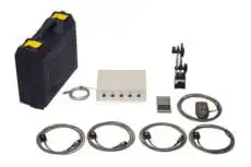
In the field this whole workflow hinges on a clean phase reference. A portable two-channel instrument such as the Balanset-1A supplies exactly that: its optical laser tachometer triggers from a small piece of reflective tape on the shaft, giving the once-per-revolution pulse that anchors each averaging window — the same pulse the instrument already uses for field balancing. With a stable trigger and a steady speed, an averaged waveform that took seconds to capture can expose a single chipped gear tooth that the raw spectrum buried entirely.

7. Advanced Variations

• Gear-synchronous averaging: triggering from the gear of interest rather than the shaft shows the mesh pattern for that specific gear, though it requires an encoder or a multi-pulse tachometer.
• Multi-order averaging: averages several orders simultaneously to separate the 1×, 2× and 3× components and give comprehensive order content.
• Difference signal: subtracting the averaged signal from the raw signal leaves a residual containing exactly what was removed — the asynchronous content — which is a useful way to expose bearing defects once the gear mesh has been stripped out.

Synchronous averaging is a sophisticated technique that dramatically enhances the visibility of periodic, speed-synchronous patterns while suppressing noise and asynchronous components. Mastering it unlocks advanced gearbox diagnostics, early defect detection in noisy environments, and clean isolation of individual component signatures inside otherwise impenetrable machinery.

---

← Back to Main Index