The Influence Coefficient Method for Field Balancing






An influence coefficient is a complex vector — carrying both an amplitude and a phase angle — that describes how a rotor system responds to a known unbalance. It captures the change in vibration at one measurement point produced by adding a known trial weight at one location on a correction plane. Put plainly, the coefficient says: “for a trial weight of this size, placed at this angle, the vibration at the bearing moved by this much and in this direction.” That single number-pair is the engine of modern field balancing.
Its great virtue is that it lets you balance a machine accurately without knowing the rotor’s physical properties — its mass, stiffness, or damping. You measure the response and let it speak for the whole system.
1. Definition: What an Influence Coefficient Represents
Vibration caused by unbalance is a vector: it has a magnitude (how much the bearing moves) and a direction (the angular position of the peak relative to the shaft, fixed by a tachometer pulse). Unbalance, likewise, is a vector — a mass at a radius and an angle. The influence coefficient is simply the ratio between them, the response per unit of applied unbalance, expressed in units such as mm/s per gram at a given radius. Because it is a ratio of two vectors it is itself a vector, and all the arithmetic of balancing is therefore vector addition and division rather than ordinary scalar maths.
2. Why the Method Is So Effective
The power of the approach is that it treats the machine as a “black box.” Rather than trying to model the rotor theoretically, it runs a practical test to measure the system’s own unique response. The benefits follow directly:
- High accuracy: it folds in every real-world dynamic effect at once — bearing stiffness, support-structure flexibility, foundation behaviour and aerodynamic forces — because all of them are already baked into the measured response.
- Versatility: it works equally for single-plane and complex multi-plane problems, on both rigid and flexible rotors.
- No disassembly: it is the standard for in-situ work, balancing a machine in its installed condition under genuine operating loads, speeds and temperatures — the state it actually runs in.
3. The Single-Plane Procedure, Step by Step
For a single-plane balance the method follows a clear, logical sequence. Each run produces one vibration vector, and the coefficient emerges from the difference between them.
- Initial run (Run 1): with the machine at normal operating conditions, measure the initial vibration vector — amplitude A₁ and phase P₁ — at the bearing. This is the response to the original unbalance, call it O.
- Trial-weight run (Run 2): stop the machine and attach a known trial weight T at a known angular position, say 0°, on the correction plane.
- Measure the new response: restart and read the new vector, amplitude A₂ and phase P₂. This is the vector sum of the original unbalance plus the trial weight’s effect, O + T.
- Find the change: the instrument performs the vector subtraction A₂ − A₁ to isolate the vector due to the trial weight alone, Teffect.
- Compute the coefficient (α): divide the trial weight’s effect by the trial weight itself — α = Teffect / T — giving the response per unit of unbalance.
- Compute the correction: to cancel the original vibration you need a weight whose effect is exactly −A₁, so the required correction weight is W = −A₁ / α.
- Install and verify: remove the trial weight, fit the calculated correction, and run again to confirm the vibration has dropped to an acceptable level.
The whole loop is just three vectors and two operations: subtract to find the trial effect, divide to find the coefficient, then divide the unwanted vibration by that coefficient to find the cure.
The vector arithmetic is easy to get wrong by hand, so most engineers let software do it. Our Influence Coefficient Calculator works the single-plane case through for you, and the Trial Weight Calculator helps size a sensible first trial mass so Run 2 produces a clear, measurable change without overstressing the rotor.
4. Multi-Plane Balancing
The same principle scales to two-plane and beyond, though the algebra grows. For a two-plane balance the instrument determines four influence coefficients — the effect of a weight in plane 1 on each of the two bearings, and the effect of a weight in plane 2 on each bearing — capturing the cross-coupling between planes. It then solves a set of simultaneous vector equations to find the correct mass and angle for both planes at once. This is what allows the technique to handle dynamic (couple) unbalance and, in principle, almost any rotating machine. For flexible rotors that bend through one or more critical speeds, the idea is extended further into modal balancing, where coefficients are measured for each significant mode.
5. Practical Conditions and Pitfalls
The method rests on one key assumption — that the system is linear and stable, so that a coefficient measured today still holds tomorrow. Several practical points follow:
- Repeatable speed: the coefficient is speed-dependent. Each run must be at the same RPM, especially near a critical speed where response changes sharply.
- A clean trial response: the trial weight must change the vibration enough to measure reliably; too small and the subtraction A₂ − A₁ is swamped by noise.
- Stable conditions: changing temperature, load or looseness shifts the true coefficient and corrupts the result — rule out such faults before balancing.
- Stored coefficients: once known for a given machine, a coefficient can be reused for a fast trim balance without a fresh trial run, the basis of single-run balancing on production rotors.
In the field this all happens inside a portable two-channel analyser. The Balanset-1A measures the 1× amplitude and phase on each run, computes the influence coefficients automatically, solves for the single- or two-plane correction, and then verifies the residual unbalance against the chosen ISO 21940-11 grade — turning the theory above into a few guided steps on site.
Coefficients That Outlive the Job
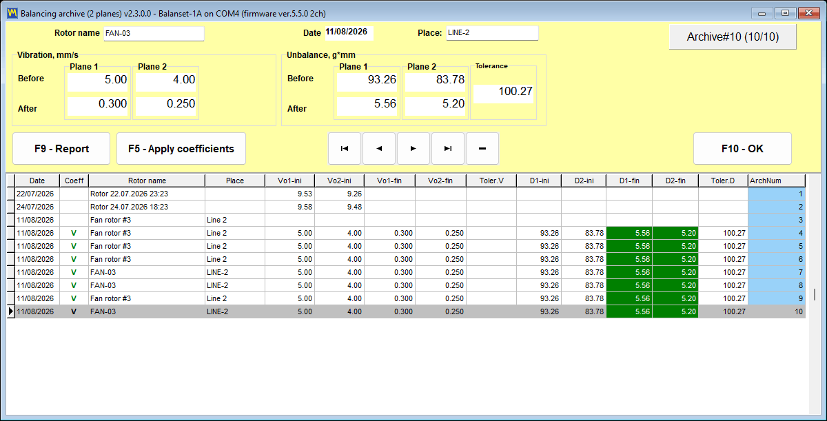
On the Balanset-1A the stored-coefficient idea is built into the session archive. Every saved balancing result carries its influence-coefficient matrix together with the trial mass, its installation radius, the fixed positions and the tolerance; records holding a reusable set are marked with a green check in the archive’s “Coeff” column.
Re-balancing the same rotor then skips the trial runs entirely: open the archive (F8), select a checked record, press “F5 – Apply coefficients” — the balancing form opens in saved-coefficients mode with the trial-run panels hidden, and a single Run 0 is enough for the program to output correction masses and angles, followed by the usual trim run.
The caveats are the ones the theory above imposes: the coefficients hold for the same machine and rotor type with unchanged sensor placement and rotation regime, and the correction angle is measured from where the trial weight stood when the coefficients were first obtained — worth marking on the rotor if reuse is planned.