ಕಂಪನ ವಿಶ್ಲೇಷಣದಲ್ಲಿ ಬೇಗ ಅರ್ಥ

ಏಕೀಕರಣ ನಲ್ಲಿ vibration ವಿಶ್ಲೇಷಣ ಕಂಪನ ಸಂಕೇತವನ್ನು ಒಂದು ಪಾರಾಮೀಟರ್ನಿಂದ ಇತರನಿಗೆ ರೂಪಾಂತರಿತ ಮಾಡುವ ಗಣಿತಶಾಸ್ತ್ರೀಯ ಪ್ರಕ್ರಿಯೆ — ಸಮಯದ ಡೋಮೈನ್ನಲ್ಲಿ ಬೇಗ ನೆರವೇರಿಸುವುದು, ಅಥವಾ, ಸಮಾನವಾಗಿ, ಆವೃತ್ತಿ ಡೋಮೈನ್ನಲ್ಲಿ ಆವೃತ್ತಿ ಮೂಲಕ ಭಾಗಿಸುವುದು। ಹೆಚ್ಚಾಗಿ ಇದು ತುಂಬುತ್ತದೆ ತ್ವರಣೆ (ಸಂವೇದಕವು ನಿಜವಾಗಿಯೂ ಕಂದುಕೊಳ್ಳುವ ಪ್ರಮಾಣ accelerometer ನಿಜವಾಗಿಯೂ) ಆಗಿ ರೂಪಾಂತರಿತ ಮಾಡುತ್ತದೆ ವೇಗ, ಅಥವಾ ವೇಗವನ್ನು ಆಗಿ ರೂಪಾಂತರಿತ ಮಾಡುತ್ತದೆ ಸ್ಥಳಾಂತರ. ಏಕೆಂದರೆ ಈ ಮೂರೂ ಕಲನಶಾಸ್ತ್ರದ ಮೂಲಕ ಸಂಯೋಜಿತವಾಗಿವೆ (ವೇಗ = ∫ ತ್ವರಣ dt; ಸ್ಥಳಾಂತರ = ∫ ವೇಗ dt), ಸಮಾಕಲನವು ಒಬ್ಬ ವಿಶ್ಲೇಷಕರಿಗೆ ಅದೇ ಕಂಪನವನ್ನು ಯಂತ್ರ, ದೋಷ ಮತ್ತು ಆವೃತ್ತಿ ವ್ಯಾಪ್ತಿಗೆ ಹೆಚ್ಚು ಸೂಕ್ತವಾದ ಯಾವ ನಿಯತಾಂಕದಲ್ಲಿ ಬೇಕಾದರೂ ವ್ಯಕ್ತಪಡಿಸಲು ಅನುಮತಿಸುತ್ತದೆ — ಮತ್ತು ಇದು ಗಣಿತೀಯ ವಿಲೋಮ ಕ್ರಿಯೆಯಾಗಿದೆ ವ್ಯುತ್ಪನ್ನೀಕರಣ.
1. ವ್ಯಾಖ್ಯಾನ: ಒಂದು ಸಂವೇದಕ, ಮೂರು ನಿಯತಾಂಕಗಳು
ಏಕೀಕರಣ ಮುಖ್ಯವಾಗಿದೆ ಏಕೆಂದರೆ ಯಾವುದೇ ಏಕ ನಿಯತಾಂಕವು ಎಲ್ಲಾ ಕಾರ್ಯಾಗಳಿಗೆ ಸರ್ವೋತ್ತಮವಲ್ಲ. ವೇಗವರ್ಧನೆಯು ಉನ್ನತ ಆವೃತ್ತಿಗಳನ್ನು ಹೈಲೈಟ್ ಮಾಡುತ್ತದೆ ಮತ್ತು ಆರಂಭಿಕ ಬೆರಿಂಗ್ ದೋಷ ಸন್ನಿವೇಶನ; ವೇಗವು ಅಂತರರಾಷ್ಟ್ರೀಯ ಯಂತ್ರ-ಕಂಪನ ಮಾನದಂಡಗಳಿಂದ ಬಳಸಲಾಗುವ ಸುಸಮತೋಲಿತ ಸಾಮಾನ್ಯ ಉದ್ದೇಶ ಮೆಟ್ರಿಕ್; ಸ್ಥಳಾಂತರ ನಿಮ್ನ ಆವೃತ್ತಿಗಳನ್ನು ಹೈಲೈಟ್ ಮಾಡುತ್ತದೆ ಮತ್ತು ನಿಧಾನ ಯಂತ್ರಗಳು ಮತ್ತು ನಿರ್ದೇಶಾಂಕ ಕೆಲಸಕ್ಕೆ ಸೂಕ್ತವಾಗಿದೆ. ಮೂರು ರೀತಿಯ ಸಂವೇದಕಗಳನ್ನು ಒದ್ದೆ ಮಾಡುವ ಬದಲಾಗಿ, ಒಬ್ಬ ಎಂಜಿನಿಯರ ವೇಗವರ್ಧನೆಯನ್ನು ಒಮ್ಮೆ ಅಳೆಯುತ್ತಾನೆ ಮತ್ತು ಇತರ ಎರಡನ್ನು ಹೊಂದಲು ಏಕೀಕರಣ ಮಾಡುತ್ತಾನೆ. ಇದೀಯೋ ಆಧುನಿಕ ವಿಶ್ಲೇಷಕವು ಒಂದೇ ಅಳತೆಯನ್ನು ವೇಗವರ್ಧನೆ, ವೇಗ ಮತ್ತು ಸ್ಥಳಾಂತರ ಎಂದು ತೋರಿಸಬಹುದು.
2. ಗಣಿತದ ಸಂಬಂಧಗಳು
ಸಮಯ-ಪ್ರದೇಶ ಏಕೀಕರಣ
- ವೇಗವರ್ಧನೆಯಿಂದ ವೇಗ: v(t) = ∫ a(t) dt
- ವೇಗದಿಂದ ಸ್ಥಳಾಂತರ: d(t) = ∫ v(t) dt
- ವೇಗವರ್ಧನೆಯಿಂದ ಸ್ಥಳಾಂತರ: d(t) = ∫∫ a(t) dt dt (double integration)
ಆವೃತ್ತಿ-ಪ್ರದೇಶ ಏಕೀಕರಣ
ದೃಶ್ಯವು ಸಂಕೇತ ಒಮ್ಮೆ ಇದರಲ್ಲಿ ಆರಂಭವಾದ ನಂತರ ಅನೇಕ ಸುಲಭವಾಗಿದೆ spectrum, ಅಲ್ಲಿ ಪ್ರತಿಯೊಂದು ಆವೃತ್ತಿ ರೇಖೆಯನ್ನು ಕೇವಲ ಸ್ಕೇಲ್ ಮಾಡಲಾಗುತ್ತದೆ:
- ವೇಗವರ್ಧನೆಯಿಂದ ವೇಗ: V(f) = A(f) / (2πf)
- ವೇಗದಿಂದ ಸ್ಥಳಾಂತರ: D(f) = V(f) / (2πf)
- ಪರಿಣಾಮ: ಆವೃತ್ತಿಯಿಂದ ಭಾಗಿಸುವುದು ನಿಮ್ನ ಆವೃತ್ತಿಗಳನ್ನು ವರ್ಧಿಸುತ್ತದೆ ಮತ್ತು ಉನ್ನತ ಆವೃತ್ತಿಗಳನ್ನು ನಿಗ್ರಹಿಸುತ್ತದೆ — ಏಕೀಕರಣ ಕುರಿತು ನೆನಪಿಟ್ಟುಕೊಳ್ಳಲು ಏಕೀಕರಣದ ಸಾಮಾನ್ಯ ಸತ್ಯ.
ಏಕೀಕರಣವು 1/f ಕಾರ್ಯಾಚರಣೆಯಾಗಿದೆ. ಇದು ಸಂಕೇತದ ನಿಮ್ನ-ಆವೃತ್ತಿ ಪರಿಧಿಯನ್ನು ವರ್ಧಿಸುತ್ತದೆ ಮತ್ತು ಉನ್ನತ-ಆವೃತ್ತಿ ಪರಿಧಿಯನ್ನು ನಿರ್ಬಂಧಿಸುತ್ತದೆ — ಇದು ನಿಖರವಾಗಿ ಅದು ವೇಗ ರೋಹಿತವು ಅದು ಬಂದ ವೇಗವರ್ಧನೆ ರೋಹಿತದೊಂದಿಗೆ ಹೋಲಿಸಿದಾಗ “ಬಾಗಿದ” ಆಗಿ ಕಾಣುವ ಯಾಕೆ.
3. ಏಕೀಕರಣ ಏಕೆ ಅಗತ್ಯವಿದೆ
ಸಂವೇದಕ ಅರ್ಥಶಾಸ್ತ್ರ
ಆಕ್ಸಿಲೆರೋಮೆಟರ್ಗಳು ಅತ್ಯಂತ ಬಹುಮುಖ ಮತ್ತು ಸಾಮಾನ್ಯವಾಗಿ ಬಳಕೆಯಲ್ಲಿರುವ ಕಂಪನ ಸಂವೇದಕಗಳಾಗಿವೆ, ಆದರೆ ತ್ವರಣವು ಸರ್ವದಾ ಸಾಕಷ್ಟು ಮಾಹಿತಿಪೂರ್ಣ ನಿಯತಾಂಕವಲ್ಲ. ಇಂಟಿಗ್ರೇಶನ್ ಮೂಲಕ ಒಂದು ಬಲಿಷ್ಠ ಆಕ್ಸಿಲೆರೋಮೆಟರ್ ಪ್ರತಿಯೊಂದು ನಿಯತಾಂಕ ಅಗತ್ಯವನ್ನೂ ನೆರವೇರಿಸಬಹುದು, ಇದು ಪೃಥಕ್ ವೇಗ ಮತ್ತು ಸ್ಥಳಾಂತರ ಸಂವೇದಕಗಳನ್ನು ಸ್ಥಾಪಿಸುವುದಕ್ಕೆ ತುಲನೆ ನೂರಾರು ಪಟ್ಟು ಸಾಕಾಣೆಮಾಡಿ.
ಆವರ್ತನದ ಮೂಲಕ ನಿಯತಾಂಕ ಆಯ್ಕೆ
- ಹೆಚ್ಚಿನ ಆವರ್ತನ (~1000 Hz ಗಿಂತ ಮೇಲೆ): ತ್ವರಣ ಉತ್ತಮ — ಇದು ಸಹ-ಸ್ಫಟಿಕ ಪ್ರಭಾವ ಮತ್ತು ಗಿಯರ್-ಮೆಶ ಶಕ್ತಿಯನ್ನು ಎತ್ತರಿಸಿ ತೋರಿಸುತ್ತದೆ.
- ಮಧ್ಯಮ ಆವರ್ತನ (10–1000 Hz): ವೇಗ ಉತ್ತಮ, ಮತ್ತು ಸಾಮಾನ್ಯ ಯಂತ್ರೋಪಕರಣ ಸ್ಥಿತಿಗೆ ಬಳಸುವ ನಿಯತಾಂಕವಾಗಿದೆ.
- ಕೆಳ ಆವರ್ತನ (~10 Hz ಕ್ಕಿಂತ ಕೆಳಗೆ): ಸ್ಥಳಾಂತರ ಉತ್ತಮ, ನಿಧಾನ ಯಂತ್ರಗಳು ಮತ್ತು ತುರತುರದ ಮೂಲ್ಯಾಂಕನಕ್ಕಾಗಿ.
- ಇಂಟಿಗ್ರೇಶನ್ ಮೂಲಕ ನೀವು ಯಾವುದೇ ಶ್ರೇಣಿಯಲ್ಲಿ ದೋಷ ಇರುವ ಸ್ಥಳಕ್ಕೆ ಸಾಕುಷ್ಠ ನಿಯತಾಂಕಕ್ಕೆ ಚಲಿಸಬಹುದು.
ಪ್ರಮಾಣ ಅವಶ್ಯಕತೆಗಳು
ಪ್ರಾಬಲ್ಯಮಾನ ಯಂತ್ರ-ಕಂಪನ ಪ್ರಮಾಣ, ISO 20816 (ಇದು ISO 10816 ಅನ್ನು ಬದಲಾಯಿಸಿತು), ನಿರ್ದಿಷ್ಟ ಮಾಡುತ್ತದೆ RMS ವೇಗ. ನೀವು ತ್ವರಣವನ್ನು ಅಳತೆ ಮಾಡಿದರೆ, ಮಿತಿಗಳ ವಿರುದ್ಧ ಹೋಲಿಸಲು ನೀವು ವೇಗಕ್ಕೆ ಸಂಯೋಜಿತ ಮಾಡಬೇಕು; ನೀವು ಸ್ಥಳಾಂತರವನ್ನು ಒಂದೊಳಗೆ ಅಳತೆ ಮಾಡಿದರೆ ಪ್ರಾಕ್ಸಿಮಿಟಿ ಪ್ರೋಬ್, ಯಾವುದೇ ವೇಗ ಹೋಲಿಕೆ ಸಿಂಧುವಾಗುವ ಮೊದಲೆ ಅದನ್ನೂ ಪರಿವರ್ತಿತ ಮಾಡಬೇಕು.
4. ಇಂಟಿಗ್ರೇಶನ್ನ ಸವಾಲುಗಳು
ಇಂಟಿಗ್ರೇಶನ್ ಗಣಿತೀಯವಾಗಿ ಸರಳವಾಗಿದೆ ಆದರೆ ಪ್ರಾಯೋಗಿಕವಾಗಿ ಕಠೋರ, ಏಕೆಂದರೆ ಉಪಯುಕ್ತ ಅದೇ 1/f ವರ್ತನೆ ಕೆಳ-ಆವರ್ತನ ತುದಿಯಲ್ಲಿ ದೋಷಗಳನ್ನೂ ವರ್ಧಿಸುತ್ತದೆ.
ಕೆಳ-ಆವರ್ತನ ಸರಿಸಲು
ಇದು ಮುಖ್ಯ ಸಮಸ್ಯೆ. ಯಾವುದೇ DC ಆಫ್ಸೆಟ್ ಅಥವಾ ಬಹಳ-ಕೆಳ-ಆವರ್ತನ ಘಟಕ ಸಣ್ಣ ಸಂಖ್ಯೆಯಿಂದ ವಿಭಾಜಿತವಾಗಿ, ಅದ್ದೇಹ ದೋಷ ನಿರ್ಮಾಣ ಮಾಡುತ್ತದೆ ಅದು ಸಂಯೋಜಿತ ಸಂಕೇತವನ್ನು ಸ್ಕೇಲ್ ಸರಿಸುವಂತೆ “ಸರಿಸಲು” ಮಾಡುತ್ತದೆ. ಪರಿಹಾರ ಒಂದು ಉನ್ನತ-ಪಾಸ್ ಫಿಲ್ಟರ್ ಇಂಟಿಗ್ರೇಶನ್ ಮೊದಲೆ ಅನ್ವಯಿಸಲಾಗುತ್ತದೆ, ಸಾಮಾನ್ಯವಾಗಿ 2–10 Hz ಕಟ್ ಆವರ್ತನ ಜೊತೆ.
ಶಬ್ದದ ವರ್ಧನೆ
ಏಕೀಕರಣವು 1/f ಕಾರ್ಯಾಚರಣೆಯಾಗಿರುವುದರಿಂದ, ಕಡಿಮೆ ಆವೃತ್ತಿಯ ಶಬ್ದವು ಆಸಕ್ತಿಯ ಸಂಕೇತಕ್ಕಿಂತ ಹೆಚ್ಚು ದೃಢವಾಗಿ ವರ್ಧಿತವಾಗುತ್ತದೆ, ಇದು ಸಂಕೇತ-ಶಬ್ದ ಅನುಪಾತವನ್ನು ಹದಡೆಯಿಡುತ್ತದೆ. ಏಕೀಕರಣದ ಮೊದಲು ಶಬ್ದವನ್ನು ಫಿಲ್ಟರ್ ಮಾಡುವುದು ಪರಿಹಾರವಾಗಿದೆ.
ದ್ವಿಮುಖ ಏಕೀಕರಣವು ಸಮಸ್ಯೆಯನ್ನು ಸಂಯೋಜಿತ ಮಾಡುತ್ತದೆ
ವೇಗವರ್ಧನೆಯಿಂದ ಸಂಪೂರ್ಣವಾಗಿ ಸ್ಥಾನಾಂತರಕ್ಕೆ ಹೋಗಲು ಎರಡು ಬಾರಿ ಏಕೀಕರಣ ಅಗತ್ಯವಾಗುತ್ತದೆ, ಆದ್ದರಿಂದ ಯಾವುದೇ DC ಆಫ್ಸೆಟ್ ಅಥವಾ ಕಡಿಮೆ-ಆವೃತ್ತಿಯ ಶಬ್ದವು ಎರಡು ಬಾರಿ ವರ್ಧಿತವಾಗುತ್ತದೆ ಮತ್ತು ದೋಷಗಳು ಗುಣಾತ್ಮಕವಾಗಿ ಬೆಳೆಯುತ್ತವೆ. ಫಲಿತಾಂಶವನ್ನು ಉಪಯೋಗಿ ಸ್ಥಿತಿಯಲ್ಲಿ ಇಡಲು ಆಕ್ರಮಣಶೀಲ ಹೆಚ್ಚಿನ-ಪಾಸ್ ಫಿಲ್ಟರಿಂಗ್ — ಸಾಮಾನ್ಯವಾಗಿ 10–20 Hz — ಅಗತ್ಯವಾಗಿದೆ.
5. ಸರಿಯಾಗಿ ಮಾಡುವುದು
ಏಕೀಕೃತ ಏಕೀಕರಣ (ವೇಗವರ್ಧನೆ → ವೇಗ)
- ಸಂಗ್ರಹಿಸಿ ಸಮರ್ಪಕ ಮಾದರಿ ದರದಲ್ಲಿ ವೇಗವರ್ಧನೆ ಸಂಕೇತ.
- DC ಆಫ್ಸೆಟ್ ತೆಗೆದುಹಾಕಿ.
- ಹೆಚ್ಚಿನ-ಪಾಸ್ ಫಿಲ್ಟರ್ ಡ್ರಿಫ್ಟ್ ನಿರ್ಮೂಲಿತ ಮಾಡಲು 2–10 Hz ನಲ್ಲಿ.
- ಸಮಾಕಲಿಸಿ (ಆವೃತ್ತಿ ಕ್ಷೇತ್ರದಲ್ಲಿ 2πf ರಿಂದ ಭಾಗಿಸಿ).
- ಪರಿಶೀಲಿಸಿ ಫಲಿತಾಂಶವು ಸುವಿವೇಚನೆಯುಕ್ತವಾಗಿರುತ್ತದೆ ಮತ್ತು ಡ್ರಿಫ್ಟ್ನಿಂದ ಮುಕ್ತವಾಗಿರುತ್ತದೆ.
ದ್ವಿಮುಖ ಏಕೀಕರಣ (ವೇಗವರ್ಧನೆ → ಸ್ಥಾನಾಂತರ)
- ಆಕ್ರಮಣಶೀಲ ಹೆಚ್ಚಿನ-ಪಾಸ್ ಫಿಲ್ಟರ್ ಅನ್ವಯ ಮಾಡಿ — ಏಕೀಕೃತ ಏಕೀಕರಣಕ್ಕಿಂತ ಹೆಚ್ಚಿನ ಕಟ್ಆಫ್ (10–20 Hz).
- ಮೊದಲ ಏಕೀಕರಣ: ವೇಗವರ್ಧನೆ → ವೇಗ.
- ಮಧ್ಯಿಕ ಪರಿಶೀಲನೆ ಮಾಡಿ ವೇಗ ಫಲಿತಾಂಶ.
- ಎರಡನೇ ಏಕೀಕರಣ: ವೇಗ → ಸ್ಥಾನಾಂತರ.
- ಅಂತಿಮ ಪರಿಶೀಲನೆ: ವಿಸ್ಥಾಪನೆ ಭೌತಿಕವಾಗಿ ಸಮಂಜಸವಾಗಿದೆ ಎಂದು ದೃಢೀಕರಿಸಿ.
6. ಆವರ್ತನ ಪ್ರಾಂತ vs. ಸಮಯ ಪ್ರಾಂತ
ಸಂಕಲನವನ್ನು ಅಮಲಿಸಲು ಎರಡು ವಿಧಾನಗಳಿವೆ, ಮತ್ತು ಆಧುನಿಕ ಯಂತ್ರಗಳು ಮಹತ್ತರ ಅಂಶದಲ್ಲಿ ಮೊದಲನೆಯದನ್ನು ಬಯಸುತ್ತವೆ.
- ಆವರ್ತನ-ಪ್ರಾಂತ ಸಂಕಲನ (ಸೂಚಿತ): ತೆಗೆದುಕೊಳ್ಳಿ FFTಪ್ರತಿಯೊಂದು ಸಾಲನ್ನು 2πf ನಿಂದ ಭಾಗಿಸಿ ಮತ್ತು ವಿಲೋಮ-ರೂಪಾಂತರ ಮಾಡಿ. ಇದು ನೇರ, ಸಂಚಿತ ದೋಷವನ್ನು ಪರಿಚಯ ಮಾಡುವುದಿಲ್ಲ, ಪೊರೆಗಳನ್ನು ತೆಗೆದುಕೊಳ್ಳುವುದನ್ನು ಸರಳ ಮಾಡುತ್ತದೆ ಮತ್ತು ಆಧುನಿಕ ವಿಶ್ಲೇಷಕಗಳಲ್ಲಿ ಪ್ರಮಾಣಿತ ವಿಧಾನವಾಗಿದೆ — ಸ್ವಚ್ಛ, ನಿಖುತ ಫಲಿತಾಂಶ ನೀಡುತ್ತದೆ.
- ಸಮಯ-ಪ್ರಾಂತ ಸಂಕಲನ: ಟ್ರೆಪೆಜಾಯಿಡಲ್ ಅಥವಾ ಸಿಂಪ್ಸನ್’ಸ್ ನಿಯಮ ಮೂಲಕ ಸಂಖ್ಯಾತ್ಮಕ ಸಂಕಲನ. ಇದು ಸಂಚಿತ ದೋಷ ಮತ್ತು ಸರಿದೋಣೆಗಳಿಂದ ಬಳಲುತ್ತದೆ ಮತ್ತು ಹೆಚ್ಚು ಜತೆಯಾಗಿ ಪೊರೆಗಳನ್ನು ಅಗತ್ಯವಿರುತ್ತದೆ, ಆದ್ದರಿಂದ ಆವರ್ತನ-ಪ್ರಾಂತ ವಿಧಾನ ಪ್ರಾಯೋಗಿಕವಾಗಿ ಸಾಧ್ಯವಿಲ್ಲದ ಸಂದರ್ಭಗಳಿಗೆ ಸಂಕ್ಷಿಪ್ತ ರಿಸರ್ವ ಮಾಡಲಾಗಿದೆ.
7. ಪ್ರಾಯೋಗಿಕ ಅನ್ವಯ ಮತ್ತು ಕ್ಷೇತ್ರ ಉಪಯೋಗ
ದಿನಾಂತರ ಕೆಲಸದಲ್ಲಿ, ಸಂಕಲನ ವಿವಿಧ ಸಂವೇದಕಗಳಿಂದ ಅಳತೆಗಳನ್ನು ಸಮಾನ ಕ್ಷೇತ್ರದಲ್ಲಿ ಹೋಲಿಕೆ ಮಾಡುವ ಅವಶ್ಯಕತೆ ನೋಡಿಸುತ್ತದೆ: ISO 20816 ಪರಿಶೀಲನೆಗಾಗಿ ವೇಗವರ್ಧಕ ಡೇಟಾವನ್ನು ವೇಗಕ್ಕೆ ಪರಿವರ್ತನೆ ಮಾಡುವುದು, ಅಥವಾ ಸಾಮೀಪ್ಯ-ಶೋಧನ ವಿಸ್ಥಾಪನೆಯನ್ನು ವೇಗಕ್ಕೆ ಪರಿವರ್ತನೆ ಮಾಡುವುದು ಹೀಗೆ ಎರಡೂ ಒಂದೇ ರೇಖಾಚಿತ್ರದಲ್ಲಿ ಕುಳಿತುಕೊಳ್ಳಬಹುದು. ನಿಧಾನ ಯಂತ್ರೋಪಕರಣಗಳಲ್ಲಿ (ಸುಮಾರು 500 RPM ಕೆಳಗೆ) ವೇಗವರ್ಧನೆ ಮತ್ತು ವೇಗ ಎರಡೂ ಚಿಕ್ಕವಾಗಿರುತ್ತವೆ, ಆದ್ದರಿಂದ ವಿಶ್ಲೇಷಕರು ಅರ್ಥಪೂರ್ಣ ಸಂಖ್ಯೆ ಪಡೆಯಲು ವಿಸ್ಥಾಪನೆಗೆ ಸಂಕಲನ ಮಾಡುತ್ತಾರೆ, ಮತ್ತು ಬಹು-ನಿಯತಾಂಕ ವಿಶ್ಲೇಷಣೆ — ಒಂದೇ ಸಂಕೇತವನ್ನು ವೇಗವರ್ಧನೆ, ವೇಗ, and ವಿಸ್ಥಾಪನೆ — ನೀಡುತ್ತದೆ ಅತ್ಯಂತ ಸಂಪೂರ್ಣ ಚಿತ್ರ ಏಕೆಂದರೆ ಪ್ರತಿಯೊಂದು ನಿಯತಾಂಕ ಆವರ್ತನ ಶ್ರೇಣಿಯ ವಿಭಿನ್ನ ಭಾಗವನ್ನು ಎತ್ತಿಹಿಡಿದುಕೊಳ್ಳುತ್ತದೆ.
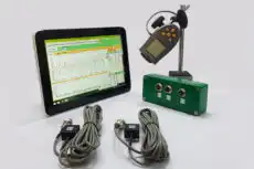
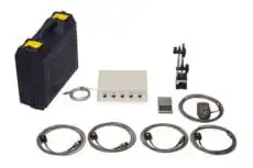
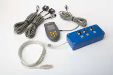
ಇದು ನಿಖರವಾಗಿ ವಾಹಕ ಯಂತ್ರ ವಾಸ್ತವ ಕೆಲಸದಲ್ಲಿ ಹೇಗೆ ವರ್ತಿಸುತ್ತದೆ. ದ್ವಿ-ಚಾನೆಲ ವಿಶ್ಲೇಷಕ ಇದೆ ಬ್ಯಾಲೆನ್ಸೆಟ್-1ಎ ಬಿಯರಿಂಗ್ ವಾಸನ್ನ ಪ್ರಮಾಣ ಸ್ಯಾಂಪಲ್ ಮಾಡುತ್ತದೆ ಮತ್ತು ISO 20816 ತೀವ್ರತೆ ಪರಿಶೀಲನೆ ಅಥವಾ 1× ಪ್ರದರ್ಶನಗಾಗಿ ವೇಗಕ್ಕೆ ಆಂತರಿಕವಾಗಿ ಸಂಕಲನ ಮಾಡುತ್ತದೆ ವೈಶಾಲ್ಯ ಮತ್ತು ಹಂತ ಅಗತ್ಯವಿರುವ field balancing — ಉಚ್ಚ-ನಿರ್ಗಮನ ಪೊರೆ ಮತ್ತು ಸಂಕಲನ ಪಾರದರ್ಶಕವಾಗಿ ಸಂಭವಿಸುತ್ತಿರುವುದರಿಂದ ಎಂಜಿನಿಯರ್ ಸರಳವಾಗಿ ಕೆಲಸಕ್ಕೆ ಹೊಂದಿಕೊಳ್ಳುವ ನಿಯತಾಂಕ ಆಯ್ಕೆ ಮಾಡುತ್ತಾರೆ.
8. ಸಾಮಾನ್ಯ ದೋಷಗಳು
- ಪೊರೆ ಇಲ್ಲದೆ ಸಂಕಲನ: ಸರಿದೋಣೆ ಮತ್ತು ಬಳಯಾಗದ ವಿಸ್ಥಾಪನೆ ಮೌಲ್ಯಗಳ ಮೋಹಿನೈಸು — ಯಾವಾಗಲೂ ಮೊದಲು ಉಚ್ಚ-ನಿರ್ಗಮನ ಪೊರೆ.
- ತಪ್ಪು ಕತ್ತರಿ ಆವರ್ತನ: ತುಂಬಾ ಕಡಿಮೆ ಹೊಂದಿಸಲಾದ ಮತ್ತು ಸರಿದೋಣೆ ಹಿಂತಿರುಗುತ್ತದೆ; ತುಂಬಾ ಹೆಚ್ಚು ಹೊಂದಿಸಲಾದ ಮತ್ತು ಮಾನ್ಯ ಲೋ-ಫ್ರಿಕ್ವೆನ್ಸಿ ವಿಷಯವಸ್ತು ತೀಳಿಸಲ್ಪಡುತ್ತದೆ. ಕತ್ತರಿ ಸರಿದೋಣೆ ತಡೆಯುವಿಕೆ ಮತ್ತು ನಡುವೆ ಸರ್ವದಾ ಸಮತೋಲನ ಆಗಿದೆ ಸಿಗ್ನಲ್ ಸಂರಕ್ಷಣೆ.
- ಮಿಶ್ರ ನಿಯತಾಂಕಗಳನ್ನು ಹೋಲಿಕೆ ಮಾಡುವುದು: ವೇಗವರ್ಧನ ಮೌಲ್ಯವನ್ನು ಎಂದಿಗೂ ವೇಗ ಮೌಲ್ಯದೊಂದಿಗೆ ನೇರವಾಗಿ ಹೋಲಿಸಬೇಡಿ — ಪ್ರಥಮ ಎರಡನ್ನೂ ಅದೇ ನಿಯತಾಂಕಕ್ಕೆ ಪರಿವರ್ತಿಸಿ, ಏಕೆಂದರೆ ಆವೃತ್ತಿ ವಿಷಯವಸ್ತು ಮಾತ್ರ ಯಾವ ನಿಯತಾಂಕ ಹೆಚ್ಚು ಓದುತ್ತದೆ ಎಂಬುದನ್ನು ಬದಲಾಯಿಸುತ್ತದೆ.
ಏಕೀಕರಣ ಒಂದು ಮೂಲಭೂತ ಸಂಕೇತ-ಸಂಸ್ಕರಣ ಕಾರ್ಯಾಚರಣೆ ಮತ್ತು ಇದು ವೇಗವರ್ಧನ, ವೇಗ ಮತ್ತು ಸ್ಥಳಾಂತರವನ್ನು ಒಂದು ಸುಸಂಗತ ವರ್ಣನೆಗೆ ಸಂಪರ್ಕಿಸುತ್ತದೆ. ಸರಿಯಾದ ಉচ್ಛ-ಪಾಸ್ ಸೋಸುವ ಮತ್ತು ಆವೃತ್ತಿ-ಕ್ಷೇತ್ರ ಅನುಷ್ಠಾನ ಸಹ ಬಳಸಿಕೊಂಡು, ಇದು ಮಾನದಂಡ ಅನುಪಾಲನ, ಸಂವೇದಕ ಆರ್ಥಿಕತೆ ಮತ್ತು ಮಾವೋ-ನಿಯತಾಂಕ ವಿಶ್ಲೇಷಣೆಗೆ ಅಡಿಪಾಯ ಹೊಂದಿದ್ದು ಇದು ಎನ್ಜಿನಿಯರರಿಗೆ ಅದಿಷ್ಟಾನ ಪ್ರವೃತ್ತಿ ನೋಡುವಾಗ ಯಾವುದೇ ನಿಯತಾಂಕದಲ್ಲಿ ಸ್ಪಷ್ಟವಾಗಿ ನೋಡಲು ಅವಕಾಶ ನೀಡುತ್ತದೆ.
