Ротор теңгерімдеудегі үш жүріс әдісін түсіну


The үш жүріс әдісі — ең кеңінен қолданылатын рәсім екі жазықтықтағы (динамикалық) теңестіруді. Ол анықтайды түзету ағындарын needed in two түзету ұстарына дәл үш өлшем жүрісін пайдалана отырып: бастапқы теңгерімсіздік жағдайын белгілейтін бір бастапқы жүріс, unbalance жағдайы, содан кейін екі дәйекті trial-weight жүрістер — әр теңгерімдеу жазықтығы үшін бір-бірден. Үш жүріс — екі жазықтықты жүйені толық сипаттауға теориялық минимум, сондықтан бұл әдіс далалық жұмыста негізгіге айналды.
Ол дәлдік пен тиімділік арасындағы тамаша тепе-теңдікті сақтайды: машинаны іске қосу мен тоқтату санын төрт жүріс әдісіне қарағанда азайта отырып, өнеркәсіптік жабдықтың басым көпшілігі үшін тиімді түзетулерді есептеуге жеткілікті деректер жинайды теңгеру tasks.
1. Үш жүріс процедурасы, қадам бойынша
Процедура қарапайым, жүйелі кезекпен жүргізіледі. Әрбір жүрісте тербеліс вектор ретінде — амплитуда мен фаза бойынша — екі тірек орнының әрқайсысында өлшенеді, себебі балансталмаудың тек мөлшерін анықтап қана қоймай, оның орнын табу үшін де екі ақпарат бөлігі қажет.
1-жүріс — Бастапқы базалық өлшеу
Машина балансталу жылдамдығында, балансталмаған, табылған күйінде жұмыс істейді. Діріл екі тірек орнында да (1-тірек және 2-тірек) өлшенеді, мыналар тіркеледі amplitude and phase angle. Бұлар бастапқы балансталмау таралуы туғызатын тербеліс векторларын білдіреді.
- 1-тіректе өлшеу: amplitude A₁, phase θ₁
- 2-тіректе өлшеу: амплитуда A₂, фаза θ₂
- Purpose: establishes the baseline condition (O₁ and O₂) that must be corrected
2-жүріс — 1-түзету жазықтығына сынақ жүк орнату
The machine is stopped and a known trial weight (T₁) is temporarily fitted at a precisely marked angular position in the first plane (typically near Bearing 1). The machine is restarted at the same speed and vibration is measured again at both bearings.
- Add: trial weight T₁ at angle α₁ in Plane 1
- 1-тіректе өлшеу: new vector (O₁ + effect of T₁)
- 2-тіректе өлшеу: new vector (O₂ + effect of T₁)
- Purpose: 1-жазықтықтағы жүктің екі тіректегі тербелісіне қалай әсер ететінін көрсетеді
Аспап мыналарды есептейді ықпал коэффициенттері 1-жазықтық үшін осы жаңа мәндерден бастапқы көрсеткіштерді векторлық алу арқылы.
3-жүріс — 2-түзету жазықтығына сынақ жүк орнату
Бірінші сынақ жүгі алынып тасталады және екінші сынақ жүгі (T₂) екінші жазықтықтағы (әдетте 2-тіректің жанында) белгіленген орынға бекітіледі. Қосымша жүрісте екі тіректегі тербеліс қайта тіркеледі.
- Remove: trial weight T₁ from Plane 1
- Add: 2-жазықтықтағы α₂ бұрышында T₂ сынақ жүгі
- 1-тіректе өлшеу: new vector (O₁ + effect of T₂)
- 2-тіректе өлшеу: жаңа вектор (O₂ + T₂ әсері)
- Purpose: 2-жазықтықтағы жүктің екі тіректегі тербелісіне қалай әсер ететінін көрсетеді
Аспапта енді әрбір жазықтықтың әрбір тіректе қалай әсер ететінін сипаттайтын төрт ықпал коэффициентінің толық жиыны бар.
2. Түзету жүктерін есептеу
Үш жүріс аяқталғаннан кейін балансталу бағдарламалық жасақтамасы орындайды вектордық математика түзету салмақтарын есептеу үшін.
Әсер коэффициенттерінің матрицасы
Үш жүргізілімнен төрт коэффициент анықталады:
- α₁₁: 1-жазықтықтың 1-мойынтіректе қалай әсер ететіні (негізгі әсер)
- α₁₂: 2-жазықтықтың 1-мойынтіректе қалай әсер ететіні (айқас байланыс)
- α₂₁: 1-жазықтықтың 2-мойынтіректе қалай әсер ететіні (айқас байланыс)
- α₂₂: 2-жазықтықтың 2-мойынтіректе қалай әсер ететіні (негізгі әсер)
Жүйені шешу
The instrument solves two simultaneous vector equations for W₁ (correction for Plane 1) and W₂ (correction for Plane 2):
- α₁₁ · W₁ + α₁₂ · W₂ = −O₁ (to cancel vibration at Bearing 1)
- α₂₁ · W₁ + α₂₂ · W₂ = −O₂ (to cancel vibration at Bearing 2)
Шешім әрбір түзету салмағы үшін қажетті массаны да, бұрыштық орынды да береді. Есептелген бұрыш кедергіге тап болғанда немесе тіркелген қалақ орындықтарының арасына түскенде, жауапты қол жетімді орындарға қайта бөлуге болады, пайдаланып бөлінген түзету деп аталады.
Final steps
- Екі сынақ салмағын да алып тастаңыз.
- Есептелген тұрақты түзету салмақтарын екі жазықтыққа да орнатыңыз.
- Тербелістің рұқсат етілген деңгейге дейін төмендегенін растау үшін тексеру жүргізілімін орындаңыз.
- Қажет болса, орындаңыз trim balance нәтижені нақтылау үшін.
3. Үш жүргізілім әдісінің артықшылықтары
Бірнеше күшті жақтары үш жүргізілімді екі жазықтықтағы теңгерімдеудің салалық стандартына айналдырды.
Оңтайлы тиімділік
Үш жүргізілім — төрт әсер коэффициентін белгілеу үшін қажетті ең аз мөлшер: бір бастапқы өлшем және әр жазықтық үшін бір сынақ жүргізілімі. Бұл жүйенің толық сипаттамасын сақтай отырып, тоқтау уақытын барынша азайтады.
Дәлелденген сенімділік
Ондаған жылдық далалық тәжірибе үш жүргізілімнің өнеркәсіптік машиналардың басым көпшілігінде сенімді теңгерімдеу үшін жеткілікті деректер беретінін дәлелдейді.
Уақыт пен шығындарды үнемдеу
Төрт жүрістік әдіспен салыстырғанда, бір сынақ жүрісін алып тастау баланстау уақытын шамамен 20%-ға қысқартады, бұл тікелей тоқтап тұру уақытының азаюына және еңбек шығындарының төмендеуіне әкеледі.
Орындау қарапайымдылығы
Жүріс саны азайған сайын сынақ тепе-теңдестіргіш салмақтармен жұмыс азаяды, қателік жіберу мүмкіндігі кемиді және деректерді басқару жеңілдейді.
Көптеген қолданбалар үшін жеткілікті
Орташа айқаспа байланысы бар және қолайлы балансировка допустері, үш жүріс тұрақты түрде сәтті нәтижелер береді.
4. Үш жүрістік әдісті қашан қолдану керек
Үш жүрістік әдіс мынадай жағдайларға сәйкес келеді:
- Кәдімгі өнеркәсіптік баланстау: электрқозғалтқыштар, желдеткіштер, сорғылар, үрлегіштер — айналмалы жабдықтардың басым бөлігі.
- Орташа дәлдік талаптары: балансировка сапасының дәрежелері қазіргі заманғы стандарт бойынша белгіленген G 2.5-тен G 16-ға дейін ISO 21940-11 (ол ұзақ уақыт танылған ISO 1940-1 өтінеулі).
- Жергілікті (орнында) баланстау қолданбалары: орын жүзінде балалау тоқтап тұру уақытын барынша азайту маңызды болған жағдайларда.
- Тұрақты механикалық жүйелер: сызықтық жауап беретін жақсы техникалық жағдайдағы жабдық.
- Стандартты ротор геометриялары: rigid rotors ұзындық пен диаметр арақатынасы типтік болған жағдайда.
5. Шектеулер және қолданбау керек жағдайлар
Кейбір жағдайларда үш жүріс жеткіліксіз болуы мүмкін.
Төрт өлшемді әдіс қашан қолданылады
- Жоғары дәлдік: өте қатаң рұқсаттар (G 0,4-тен G 1,0-ге дейін), мұнда төртінші өлшемнің қосымша сызықтылық тексеруі маңызды мәнге ие болады.
- Күшті айқасқан байланыс: түзету жазықтықтары өте жақын орналасқан немесе жоғары асимметриялы жүйелер stiffness.
- Жүйе сипаттамалары белгісіз: ерекше немесе арнайы жабдықты алғаш рет теңгерімдеу.
- Проблемалы жабдық: сызықтық емес мінез-құлық немесе механикалық ақаулар белгілері бар жабдық.
Бір жазықтықтағы теңгерімдеу жеткілікті болатын жағдайлар
- Динамикалық дисбалансы минималды болатын жіңішке, диск тәрізді роторлар.
- Тек бір подшипник орнында айтарлықтай дірілдің байқалатын жағдайлары.
6. Басқа әдістермен салыстыру
Үш өлшемді және төрт өлшемді әдістерді салыстыру
| Aspect | Three-Run | Four-Run |
|---|---|---|
| Number of runs | 3 (бастапқы + 2 сынақ) | 4 (бастапқы + 2 сынақ + біріктірілген) |
| Time required | Shorter | ~20% longer |
| Сызықтылықты тексеру | No | Иә (4-өлшем тексереді) |
| Типтік қолданыс салалары | Жалпы өндірістік жұмыстар | Жоғары дәлдіктегі, маңызды жабдық |
| Accuracy | Жақсы | Excellent |
| Complexity | Lower | Higher |
Үш жүріс әдісі мен бір жазықтықтағы балансировка әдісін салыстыру
Үш жүріс әдісі іргелі түрде ерекшеленеді бір жазықтықтағы балансировка, ол тек екі жүрісті (бастапқы және бір сынақ жүрісі) пайдаланады, бірақ тек бір түзету жазықтығын ғана түзете алады және мынаны жоя алмайды жұп дисбаланс. Ротордың екі ұшы дербес теңгерімсіздік тудыра алатындай ұзын болған жағдайда екі жазықтықта жұмыс — демек үш жүріс әдісі — міндетті түрде қолданылады.
7. Жетістікке жету үшін үздік тәжірибелер
Сынақ салмақтарын таңдау
- Тербеліс амплитудасын 25–50% өзгертетін сынақ салмақтарын таңдаңыз.
- Тым аз: сигнал/шу қатынасы нашар және есептеу қателіктері туындайды.
- Тым үлкен: сызықтық емес жауап немесе қауіпті тербеліс деңгейінің қаупі бар.
- Өлшеу сапасының тұрақтылығын қамтамасыз ету үшін екі жазықтықта да ұқсас өлшемдегі салмақтарды пайдаланыңыз. А пробалық салмақты есептегіш ротор массасы мен айналу жылдамдығы бойынша дәл бірінші бағалауды береді.
Жұмыс жағдайларының тұрақтылығы
- Үш жүрістің барлығында бірдей айналу жылдамдығын сақтаңыз.
- Қажет болған жағдайда жүрістер арасында жылулық тұрақтануды қамтамасыз етіңіз.
- Технологиялық жағдайларды — ағынды, қысымды, температураны — тұрақты ұстаңыз.
- Датчиктердің бірдей орналасуын және бекіту тәсілдерін пайдаланыңыз.
Data quality
- Әр жүрісте бірнеше өлшеу жүргізіп, орташа мәнді есептеңіз.
- Фаза өлшемдерінің тұрақты және қайталанатынын тексеріңіз.
- Сынақ салмақтары анық өлшенетін өзгерістер тудыратынын тексеріңіз.
- Өлшеу қатесін көрсететін ауытқуларды бақылаңыз.
Орнату дәлдігі
- Сынақ салмақтарының бұрыштық орындарын мұқият белгілеп, тексеріңіз.
- Сынақ салмақтары берік бекітілгенін және жұмыс барысында жылжымайтынын тексеріңіз.
- Түзету салмақтарын да сол мұқияттылықпен орнатыңыз.
- Тексеру жүрісіне дейін массалар мен бұрыштарды қайта тексеріңіз.
8. Жиі кездесетін мәселелерді жою
Түзетуден кейінгі нашар нәтижелер
Ықтимал себептер:
- Түзету салмақтары дұрыс емес бұрыштарда немесе дұрыс емес массалармен орнатылған.
- Жұмыс жағдайлары сынақ жүрістері мен түзету орнату арасында өзгерді.
- Механикалық ақаулар — looseness, misalignment — теңгеруге дейін жойылмаған.
- Жүйенің сызықтық емес жауабы.
Сынақ салмақтары аз жауап береді
Solutions:
- Үлкенірек сынақ салмақтарын пайдаланыңыз немесе оларды үлкен радиусқа орналастырыңыз.
- Датчикті орнатуды және сигнал сапасын тексеріңіз.
- Жұмыс жиілігінің дұрыс екенін тексеріңіз.
- Жүйенің өте жоғары болып табылатынын қарастырыңыз damping немесе төмен жауап сезімталдығын.
Тұрақсыз өлшемдер
Solutions:
- Жылулық және механикалық тұрақтануға қосымша уақыт беріңіз.
- Датчикті бекітуді жақсартыңыз — магниттердің орнына шпилькаларды қолданыңыз.
- Сыртқы тербеліс көздерінен оқшаулаңыз.
- Тұрақсыз жұмыс режиміне себеп болатын механикалық ақауларды жойыңыз.
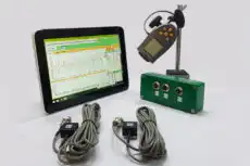
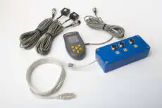
9. Өндірістік жағдайда үш жүріс әдісі
Балансировка станогын қажет етпейтіндіктен және тек бірнеше іске қосуды талап ететіндіктен, үш жүріс әдісі портативті аспаппен орнында балансировка жасауға өте қолайлы. Қос арналы анализатор, мысалы Балансет-1А бір жүріс кезінде екі тіректегі амплитуда мен фазаны оқиды, ықпал коэффициенттерін автоматты түрде есептейді және әрбір түзету салмағы үшін масса мен бұрышты қайтарады — содан кейін салмақтар орнатылғаннан кейін нәтижені қалдық дисбалансы таңдалған ISO 21940-11 сыныбымен салыстырып тексереді. Жұмыс жылдамдығында машинаның өз тіректерінде жұмыс істей отырып, ол ротордың нақты жұмыс жағдайын тіркейді, дәл осы нәрсе үш жүріс әдісін өндірістік жағдайда сенімді етеді field balancing.
