రోటర్ బ్యాలెన్సింగ్లో వెక్టర్ కూడికెను అర్థం చేసుకోవడం

వెక్టర్ సంకలనం రెండు లేదా అంతకంటే ఎక్కువ వెక్టర్లను ఒకే resultant వెక్టర్గా కలిపే గణిత పద్ధతి. rotor balancing, కంపనాన్ని ఒక వెక్టర్గా పరిగణిస్తారు, ఎందుకంటే అది ఒకేసారి రెండు సమాచారాలను కలిగి ఉంటుంది: ఒక పరిమాణం (దాని amplitude) మరియు ఒక దిశ (దాని phase angle). ఇది చాలా ముఖ్యమైనది, ఎందుకంటే వేర్వేరు మూలాల unbalance combine vectorially, బీజగణితంగా కాదు — వాటి phase సంబంధాలు వాటి పరిమాణాల వలె అంతే ముఖ్యమైనవి. అందువల్ల వెక్టర్ కూడికెపై దృఢమైన అవగాహన ఉండటం వల్ల ఒక ఇంజినీర్ బ్యాలెన్సింగ్ డేటాను సరిగ్గా చదవగలరు మరియు ఒక correction weight మొత్తం రోటర్ వ్యవస్థ యొక్క కంపనాన్ని ఎలా మార్చుతుందో అంచనా వేయగలరు.
1. కంపనాన్ని వెక్టర్గా ఎందుకు పరిగణించాలి
అసమతుల్యత వల్ల ఉత్పన్నమయ్యే కంపనం ఒక తిరిగే బలం, ఇది ప్రతి విప్పు సరిగ్గా ఒకసారి పునరావృతమవుతుంది. ఏదైనా సెన్సార్ స్థానంలో కొలిచినప్పుడు దానికి రెండు విడదీయలేని లక్షణాలు ఉంటాయి:
- Amplitude: చలనం యొక్క పరిమాణం లేదా తీవ్రత, సాధారణంగా mm/s, in/s లేదా microns లో వ్యక్తం చేయబడుతుంది.
- Phase: రోటర్పై reference మార్కుకు సంబంధించి శిఖరం సంభవించే కోణీయ క్షణం, 0° నుండి 360° వరకు డిగ్రీలలో చదవబడుతుంది మరియు keyphasor pulse.
phase నిర్ణాయకమైనది కావున, కంపన amplitudeలను ఎప్పుడూ సరళంగా కూడలేరు. రెండు అసమతుల్యతలు ఒక్కొక్కటి 5 mm/s ఉత్పత్తి చేస్తాయని ఊహించండి: వాటి మధ్య కోణాన్ని బట్టి మొత్తం 0 mm/s — అవి 180° అంతరంలో ఉండి రద్దు చేసుకుంటే — నుండి 10 mm/s వరకు ఏదైనా కావచ్చు, అవి ఒకే phase లో ఉండి బలోపేతమైతే. కోణాన్ని బట్టి మధ్యలో ఏదైనా సాధ్యమే. వెక్టర్ కూడికె మాత్రమే, amplitude మరియు phase రెండింటినీ పరిగణిస్తూ, సరైన సమాధానాన్ని ఇస్తుంది.
2. వెక్టర్ కూడికె యొక్క గణిత ఆధారం
ఒక వెక్టర్ను రెండు సమానమైన రూపాలలో వ్రాయవచ్చు, మరియు బ్యాలెన్సింగ్ రెండింటినీ ఉపయోగిస్తుంది, వాటి మధ్య స్వేచ్ఛగా మార్చుకుంటుంది.
ధ్రువ రూపం (పరిమాణం మరియు కోణం)
ఇక్కడ వెక్టర్ ఒక amplitude ఎ ఒక దశ కోణంలో θ — ఉదాహరణకు, 5.0 mm/s ∠ 45°. ఇది సాంకేతిక నిపుణుడికి అత్యంత సహజమైన రూపం, ఎందుకంటే ఇది పరికరం ప్రదర్శించే దానికి మరియు ఒక polar plot.
దీర్ఘచతురస్రాకార (కార్తీజియన్) రూపం (X మరియు Y భాగాలు)
ఇక్కడ వెక్టర్ను త్రికోణమితిని ఉపయోగించి ఒక క్షితిజ సమాంతర (X) మరియు నిలువు (Y) భాగంగా విభజిస్తారు:
- X = A × cos(θ)
- Y = A × sin(θ)
అప్పుడు కూడికె చాలా సులభమవుతుంది: అన్ని X భాగాలను కూడండి, అన్ని Y భాగాలను కూడండి, మరియు మీకు resultant’s భాగాలు లభిస్తాయి, వాటిని పరిమాణం-మరియు-కోణం సమాధానం కావాలన్నప్పుడు ధ్రువ రూపంలోకి మార్చవచ్చు.
ఒక పని చేయబడిన ఉదాహరణ
రెండు కంపన వెక్టర్లను తీసుకోండి:
- వెక్టర్ 1: 4.0 mm/s ∠ 30°
- వెక్టర్ 2: 3.0 mm/s ∠ 120°
ప్రతిదాన్ని దీర్ఘచతురస్రాకార రూపంలోకి మార్చండి:
- Vector 1: X₁ = 4.0 × cos(30°) = 3.46, Y₁ = 4.0 × sin(30°) = 2.00
- Vector 2: X₂ = 3.0 × cos(120°) = −1.50, Y₂ = 3.0 × sin(120°) = 2.60
భాగాలను కూడండి:
- X_total = 3.46 + (−1.50) = 1.96
- Y_total = 2.00 + 2.60 = 4.60
తిరిగి ధ్రువ రూపంలోకి మార్చండి:
- Amplitude = √(1.96² + 4.60²) = 5.00 mm/s
- Phase = arctan(4.60 / 1.96) = 66.9°
ఫలితం: కలిసిన కంపనం 5.00 mm/s ∠ 66.9°. గమనించండి: 4.0 మరియు 3.0 mm/s యొక్క రెండు వెక్టర్లు 7.0కి not కూడలేదు; అవి 90° అంతరంలో ఉన్నందున అవి సరిగ్గా 5.0కి కలిశాయి, సుపరిచిత 3-4-5 లంబ త్రిభుజం. అసలు కూడికె మరియు నిజమైన ఫలితం మధ్య ఆ వ్యత్యాసమే phase ని ఎందుకు విస్మరించలేమో స్పష్టంగా చెప్తుంది. మీరు మీ స్వంత కొలిచిన వెక్టర్లను చేతి అంకగణితం లేకుండా కలపాలనుకుంటే, కంపన దశ కోణం కాల్క్యులేటర్ నేరుగా మార్పిడి మరియు కూడికను నిర్వహిస్తుంది.
3. గ్రాఫికల్ టిప్-టు-టెయిల్ పద్ధతి
వెక్టార్ కూడికను రేఖాచిత్రం ద్వారా కూడా చేయవచ్చు, ఇది వెక్టార్లు ఎలా కలుపుతాయో అనే విషయంలో తక్షణ దృశ్య అనుభవాన్ని ఇస్తుంది మరియు పోలార్ ప్లాట్లో సులభంగా స్కెచ్ చేయవచ్చు:
- మొదటి వెక్టార్ను గీయండి: మూలం నుండి, దాని పొడవు amplitude కు మరియు దాని దిశ phase కు అనుగుణంగా సెట్ చేయబడుతుంది.
- రెండవ వెక్టార్ను స్థానంలో ఉంచండి: దాని తోక (tail) ను మొదటి వెక్టార్ చివర (tip) వద్ద ఉంచండి, దాని స్వంత సరైన పొడవు మరియు కోణాన్ని అలాగే ఉంచుతూ.
- ఫలిత వెక్టార్ను గీయండి: మూలం నుండి రెండవ వెక్టార్ చివరకు గీసిన రేఖ మొత్తాన్ని సూచిస్తుంది.
ఈ నిర్మాణం correction weight ను జోడించడం లేదా తొలగించడం వల్ల కలిగే ప్రభావాన్ని త్వరగా అంచనా వేయడానికి మరియు పరికరం ఉత్పత్తి చేసే సంఖ్యలను ధృవీకరించుకోవడానికి చాలా ఉపయోగకరంగా ఉంటుంది.
4. బ్యాలెన్సింగ్లో ఆచరణాత్మక అనువర్తనం
వెక్టార్ కూడిక అనేది ఒక పక్క లెక్క కాదు — ఇది బ్యాలెన్సింగ్ వర్క్ఫ్లో యొక్క ప్రతి దశలోనూ అల్లుకొని ఉంటుంది.
అసలు unbalance మరియు trial weight ను కలపడం
When a trial weight అమర్చినప్పుడు, కొత్త రీడింగ్ అనేది అసలు unbalance vibration (O) మరియు trial weight’s effect (T) యొక్క వెక్టార్ మొత్తం. పరికరం (O+T) ని నేరుగా కొలుస్తుంది; T ను వేరుచేయడానికి అది వెక్టార్ వ్యవకలనాన్ని నిర్వహిస్తుంది: T = (O+T) − O.
ప్రభావ గుణకం గణన
The influence coefficient trial weight యొక్క వెక్టార్ ప్రభావాన్ని trial mass తో భాగించడం ద్వారా కనుగొనబడుతుంది, కాబట్టి ఇది కూడా ఒక వెక్టార్ పరిమాణం — ఒక నిర్దిష్ట కోణంలో, బరువు యూనిట్కు vibration మొత్తం. The ఇన్ఫ్లుయెన్స్ కోఎఫిషియెంట్ కాలిక్యులేటర్ ఈ single-plane కేసును స్వయంచాలకంగా నిర్వహిస్తుంది.
దిద్దుబాటు బరువు నిర్ణయం
correction weight వెక్టార్ అనేది అసలు vibration యొక్క ప్రతికూల (180° phase shift) వెక్టార్, influence coefficient తో భాగించబడుతుంది. ఈ విధంగా పరిమాణం నిర్ణయించినప్పుడు, దాని ప్రభావం — అసలు unbalance కు వెక్టార్గా కలిపినప్పుడు — దాన్ని రద్దు చేస్తుంది, vibration ను సున్నా వైపుకు నెట్టుతుంది.
చివరి కంపనాన్ని అంచనా వేయడం
correction అమర్చిన తర్వాత, అంచనా వేయబడిన అవశేష కంపనం అసలు vibration వెక్టార్కు correction యొక్క లెక్కించిన ప్రభావాన్ని కలిపి అంచనా వేయవచ్చు. ఆ అంచనాను కొలవబడిన ఫలితంతో పోల్చడం మొత్తం పని నాణ్యతను తనిఖీ చేయడానికి శక్తివంతమైన పద్ధతి.
5. వెక్టర్ వ్యవకలనం
వెక్టార్ వ్యవకలనం అనేది రెండవ వెక్టార్ను తిప్పికొట్టడంతో (180° తిప్పడం) వెక్టార్ కూడిక మాత్రమే. వెక్టార్ A నుండి వెక్టార్ B ను వ్యవకలనం చేయడానికి:
- B ని 180° తిప్పడం ద్వారా తిప్పికొట్టండి — లేదా, దీర్ఘచతురస్రాకార రూపంలో, దాని రెండు భాగాలను కేవలం నిరాకరించండి.
- తిప్పికొట్టిన B ని A కి సాధారణ వెక్టార్ కూడికతో కలపండి.
పైన పేర్కొన్నట్లు, ఇది trial weight యొక్క ప్రభావాన్ని వేరుచేసే ఆపరేషన్, T = (O+T) − O, ఇక్కడ O అనేది అసలు vibration మరియు (O+T) అనేది trial weight అమర్చిన తర్వాత రీడింగ్.
6. సాధారణ తప్పులు మరియు అపోహలు
వెక్టార్ గణితానికి సంబంధించిన చాలా బ్యాలెన్సింగ్ లోపాలు మూడు వలలలో పడతాయి:
- వ్యాప్తులను నేరుగా కూడడం: 3 mm/s + 4 mm/s ని 7 mm/s గా భావించడం phase ను పూర్తిగా విస్మరిస్తుంది; పని చేసిన ఉదాహరణ చూపినట్లు, నిజమైన ఫలితం వాటి మధ్య కోణంపై ఆధారపడి ఉంటుంది.
- దశ సమాచారాన్ని విస్మరించడం: phase reference లేకుండా, amplitude మాత్రమే ఆధారంగా బ్యాలెన్స్ చేయడానికి ప్రయత్నించడం దాదాపు ఎప్పుడూ మంచి ఫలితానికి చేరదు.
- కోణ నిర్వచన అసంగతత: సవ్యదిశ మరియు అపసవ్యదిశ సంప్రదాయాలను కలపడం, లేదా తప్పు reference నుండి కొలవడం, correction weights ను rotor లో తప్పు స్థానానికి పంపుతుంది.
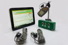
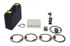
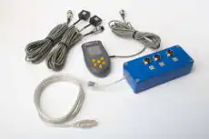
7. ఆధునిక పరికరాలు వెక్టార్ గణితాన్ని నిర్వహిస్తాయి
గణితాన్ని అర్థం చేసుకోవడం ఏ బ్యాలెన్సింగ్ నిపుణుడికైనా అవసరమైనప్పటికీ, అంకగణిత లెక్కలు ఇప్పుడు పరికరం ద్వారా స్వయంచాలకంగా నిర్వహించబడతాయి. ఇలాంటి పోర్టబుల్ అనాలైజర్ Balanset-1A రెండు చానెల్ల నుండి amplitude మరియు phase సేకరిస్తుంది, అన్ని వెక్టర్ అదనం, వ్యవకలనం మరియు భాగహారాలను అంతర్గతంగా నిర్వహిస్తుంది, ఫలితాలను సంఖ్యాత్మకంగా మరియు polar plots పై గ్రాఫికల్గా ప్రదర్శిస్తుంది, మరియు అమర్చడానికి సిద్ధంగా ఉన్న తుది correction weight యొక్క ద్రవ్యరాశి మరియు కోణ స్థానాన్ని నివేదిస్తుంది. అయినప్పటికీ, అంతర్లీన సిద్ధాంతం ఇంకా విలువైనదే: దాన్ని అర్థం చేసుకున్న ఇంజనీర్ పరికరం’s అవుట్పుట్ను ధృవీకరించగలడు, ఫలితం తప్పుగా కనిపించినప్పుడు అసాధారణతలను నిర్ధారించగలడు, మరియు కొన్ని బ్యాలెన్సింగ్ వ్యూహాలు ఇతరులకంటే వేగంగా ఎందుకు కలుస్తాయో అర్థం చేసుకోగలడు.
