Field Balancing కోసం Influence Coefficient Method


An influence coefficient ఒక సంక్లిష్టమైన వెక్టర్ — amplitude మరియు ఒక phase కోణం — రెండూ కలిగి, ఒక తెలిసిన దానికి rotor system ఎలా స్పందిస్తుందో వర్ణిస్తుంది unbalance. అది vibration ఒక కొలత బిందువు వద్ద తెలిసిన trial weight లో ఒక స్థానంలో మార్పును గ్రహిస్తుంది కరెక్షన్ ప్లేన్. సరళంగా చెప్పాలంటే, coefficient ఇలా చెప్తుంది: “ఈ పరిమాణంలో, ఈ కోణంలో ఉంచిన trial weight కోసం, bearing వద్ద vibration ఇంత మేర, ఈ దిశలో మారింది.” ఆ ఒక్క సంఖ్య-జంట ఆధునిక field balancing.
దీని గొప్ప లక్షణం ఏమిటంటే, ఇది మిమ్మల్ని ఒక యంత్రాన్ని ఖచ్చితంగా balance చేయడానికి అనుమతిస్తుంది without rotor యొక్క భౌతిక లక్షణాలు — దాని ద్రవ్యరాశి, stiffness, లేదా damping తెలియకుండానే. మీరు response ను కొలచి, అది మొత్తం system కోసం మాట్లాడనివ్వండి.
1. నిర్వచనం: Influence Coefficient దేన్ని సూచిస్తుంది
unbalance వల్ల కలిగే vibration ఒక వెక్టర్: దానికి ఒక magnitude (bearing ఎంత కదులుతుంది) మరియు ఒక దిశ (shaft కు సంబంధించిన peak యొక్క కోణీయ స్థానం, ఒక tachometer పల్స్ ద్వారా నిర్ణయించబడింది) ఉంటాయి. unbalance కూడా ఒక వెక్టర్ — ఒక radius మరియు కోణంలో ఒక ద్రవ్యరాశి. influence coefficient అనేది వాటి మధ్య నిష్పత్తి మాత్రమే, అంటే వర్తింపజేసిన unbalance యొక్క unit కు response, ఇచ్చిన radius వద్ద mm/s per gram వంటి యూనిట్లలో వ్యక్తీకరించబడుతుంది. ఇది రెండు వెక్టర్ల నిష్పత్తి కాబట్టి, ఇది స్వయంగా ఒక వెక్టర్, మరియు balancing యొక్క మొత్తం గణితం అందువల్ల vector addition మరియు సాధారణ scalar గణితానికి బదులు భాగహారం అవుతుంది.
2. ఈ Method ఎందుకు అంత ప్రభావవంతంగా ఉంటుంది
ఈ విధానం యొక్క శక్తి ఏమిటంటే, ఇది యంత్రాన్ని ఒక “black box” గా పరిగణిస్తుంది. rotor ను సైద్ధాంతికంగా నమూనా చేయడానికి ప్రయత్నించే బదులు, system యొక్క ప్రత్యేక response ను కొలవడానికి ఒక ఆచరణాత్మక పరీక్ష నిర్వహిస్తుంది. ప్రయోజనాలు నేరుగా అనుసరిస్తాయి:
- అధిక ఖచ్చితత్వం: ఇది ఒకేసారి ప్రతి నిజ-ప్రపంచ డైనమిక్ ప్రభావాన్ని చేర్చుకుంటుంది — బేరింగ్ దృఢత్వం, సపోర్ట్ నిర్మాణ సౌలభ్యం, పునాది ప్రవర్తన మరియు aerodynamic forces — ఎందుకంటే అవన్నీ ఇప్పటికే కొలిచిన స్పందనలో చేర్చబడి ఉంటాయి.
- Versatility: ఇది సమానంగా పని చేస్తుంది single-plane and complex multi-plane సమస్యలు, రెండింటిలోనూ rigid and flexible rotors.
- విడదీయకుండా: ఇది in-situ పనికి ప్రమాణం — నిజమైన ఆపరేటింగ్ లోడ్లు, వేగాలు మరియు ఉష్ణోగ్రతల కింద యంత్రాన్ని దాని ఇన్స్టాల్ చేసిన స్థితిలో బ్యాలెన్స్ చేయడం — అది వాస్తవంగా పని చేసే స్థితి.
3. సింగిల్-ప్లేన్ విధానం, దశల వారీగా
సింగిల్-ప్లేన్ బ్యాలెన్సింగ్ కోసం, ఈ పద్ధతి స్పష్టమైన, తార్కిక క్రమాన్ని అనుసరిస్తుంది. ప్రతి రన్ ఒక vibration వెక్టార్ను ఉత్పత్తి చేస్తుంది, మరియు కోఎఫిషియెంట్ వాటి మధ్య వ్యత్యాసం నుండి వస్తుంది.
- ప్రారంభ రన్ (రన్ 1): యంత్రం సాధారణ ఆపరేటింగ్ పరిస్థితుల్లో ఉన్నప్పుడు, బేరింగ్ వద్ద ప్రారంభ vibration వెక్టార్ను కొలవండి — amplitude A₁ మరియు phase P₁. ఇది అసలు unbalance కు స్పందన, దీన్ని O అని పిలుద్దాం.
- ట్రయల్ వెయిట్ రన్ (రన్ 2): యంత్రాన్ని ఆపి, కరెక్షన్ ప్లేన్లో తెలిసిన కోణ స్థానంలో, అంటే 0°లో, తెలిసిన trial weight T ని అమర్చండి.
- కొత్త స్పందనను కొలవండి: మళ్ళీ ప్రారంభించి కొత్త వెక్టార్ను చదవండి, amplitude A₂ మరియు phase P₂. ఇది అసలు unbalance మరియు trial weight’s ప్రభావం యొక్క వెక్టార్ మొత్తం, O + T.
- మార్పును గుర్తించండి: పరికరం trial weight వల్ల మాత్రమే వచ్చే వెక్టార్ను వేరుపరచడానికి వెక్టార్ వ్యవకలనం A₂ − A₁ చేస్తుంది, Teffect.
- కోఎఫిషియెంట్ (α) లెక్కించండి: trial weight’s ప్రభావాన్ని trial weight తో భాగించండి — α = Teffect / T — unbalance యొక్క ప్రతి యూనిట్కు స్పందన ఇవ్వడం.
- కరెక్షన్ లెక్కించండి: అసలు vibration ని రద్దు చేయడానికి మీకు −A₁ కు సమానమైన ప్రభావం ఉన్న weight అవసరం, కాబట్టి అవసరమైన correction weight is W = −A₁ / α.
- ఇన్స్టాల్ చేసి ధృవీకరించండి: trial weight తొలగించి, లెక్కించిన correction weight అమర్చి, vibration అంగీకార్హమైన స్థాయికి తగ్గిందని నిర్ధారించడానికి మళ్ళీ రన్ చేయండి.
మొత్తం లూప్ కేవలం మూడు వెక్టార్లు మరియు రెండు ఆపరేషన్లు మాత్రమే: trial ప్రభావాన్ని కనుగొనడానికి వ్యవకలనం చేయండి, కోఎఫిషియెంట్ కనుగొనడానికి భాగించండి, తర్వాత పరిష్కారాన్ని కనుగొనడానికి అవాంఛిత vibration ని ఆ కోఎఫిషియెంట్తో భాగించండి.
వెక్టార్ అంకగణితాన్ని చేత్తో చేస్తే తప్పు చేయడం సులభం, కాబట్టి చాలా మంది ఇంజనీర్లు సాఫ్ట్వేర్తో చేయిస్తారు. మా ఇన్ఫ్లుయెన్స్ కోఎఫిషియెంట్ కాలిక్యులేటర్ సింగిల్-ప్లేన్ కేసును మీ కోసం పూర్తి చేస్తుంది, మరియు ట్రయల్ వెయిట్ కాల్క్యులేటర్ సహేతుకమైన మొదటి trial mass యొక్క పరిమాణాన్ని నిర్ణయించడానికి సహాయపడుతుంది, తద్వారా రన్ 2 రోటర్ను అతిగా ఒత్తిడికి గురి చేయకుండా స్పష్టమైన, కొలవగలిగే మార్పును ఉత్పత్తి చేస్తుంది.
4. మల్టీ-ప్లేన్ బ్యాలెన్సింగ్
అదే సూత్రం రెండు-ప్లేన్ మరియు అంతకు మించి వర్తించవచ్చు, అయినప్పటికీ బీజగణితం పెరుగుతుంది. ఒక రెండు-తలాల బ్యాలెన్సింగ్ పరికరం నిర్ణయిస్తుంది four influence coefficients — ప్లేన్ 1 లో weight యొక్క ప్రభావం రెండు బేరింగ్లలో ప్రతిదానిపైనా, మరియు ప్లేన్ 2 లో weight యొక్క ప్రభావం ప్రతి బేరింగ్పైనా — ప్లేన్ల మధ్య cross-coupling ను గ్రహించడం. ఇది తర్వాత రెండు ప్లేన్లకు ఒకేసారి సరైన mass మరియు కోణాన్ని కనుగొనడానికి ఏకకాల వెక్టార్ సమీకరణాల సమితిని సాధిస్తుంది. ఈ సాంకేతికత ఏమిటంటే దానిని నిర్వహించడానికి అనుమతిస్తుంది డైనమిక్ (కపుల్) unbalance మరియు, సూత్రపరంగా, దాదాపు ఏదైనా తిరిగే యంత్రం. ఒకటి లేదా అంతకంటే ఎక్కువ critical speeds ద్వారా వంగే flexible rotors కోసం, ఆలోచనను మరింత విస్తరించారు మోడల్ బ్యాలెన్సింగ్, ఇక్కడ ప్రతి ముఖ్యమైన మోడ్కు కోఎఫిషియెంట్లు కొలవబడతాయి.
5. ఆచరణాత్మక పరిస్థితులు మరియు లోపాలు
ఈ పద్ధతి ఒక కీలక అనుమానంపై ఆధారపడుతుంది — సిస్టమ్ రేఖీయంగా మరియు స్థిరంగా, తద్వారా నేడు కొలిచిన కోఎఫిషియెంట్ రేపటికి కూడా చెల్లుబాటు అవుతుంది. అనేక ఆచరణాత్మక అంశాలు అనుసరిస్తాయి:
- పునరావృత వేగం: గుణకం వేగంపై ఆధారపడి ఉంటుంది. ప్రతి రన్ అదే RPM వద్ద ఉండాలి, ముఖ్యంగా ఒక సమీపంలో critical speed ప్రతిస్పందన తీవ్రంగా మారే చోట.
- స్పష్టమైన ట్రయల్ ప్రతిస్పందన: పరీక్ష బరువు కంపనాన్ని విశ్వసనీయంగా కొలవగలిగేటంత మార్పు చేయాలి; చాలా చిన్నగా ఉంటే A₂ − A₁ వ్యవకలనం శబ్దంలో మునిగిపోతుంది.
- స్థిర పరిస్థితులు: మారుతున్న ఉష్ణోగ్రత, భారం లేదా looseness నిజమైన గుణకాన్ని మార్చి ఫలితాన్ని దెబ్బతీస్తుంది — బ్యాలెన్సింగ్కు ముందు అలాంటి లోపాలను తొలగించండి.
- నిల్వ చేసిన గుణకాలు: ఒక నిర్దిష్ట యంత్రం కోసం తెలిసినప్పుడు, వేగవంతమైన పనికి ఒక గుణకాన్ని మళ్ళీ ఉపయోగించవచ్చు trim balance కొత్త పరీక్ష రన్ లేకుండా, ఉత్పత్తి రోటర్లపై సింగిల్-రన్ బ్యాలెన్సింగ్ ఆధారం.
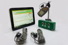
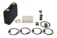
క్షేత్రంలో ఇవన్నీ ఒక పోర్టబుల్ రెండు-ఛానల్ విశ్లేషకంలో జరుగుతాయి. ది Balanset-1A ప్రతి రన్లో 1× మోతాదు మరియు దశను కొలుస్తుంది, ప్రభావ గుణకాలను స్వయంచాలకంగా లెక్కిస్తుంది, సింగిల్- లేదా టూ-ప్లేన్ దిద్దుబాటును పరిష్కరిస్తుంది, ఆపై అవశేష అసమతుల్యత ఎంచుకున్న ISO 21940-11 గ్రేడ్కు వ్యతిరేకంగా — పై సిద్ధాంతాన్ని సైట్లో కొన్ని మార్గదర్శిత దశలుగా మారుస్తుంది.
