ਵਾਟਰਫਾਲ ਪਲਾਟ (ਕੈਸਕੇਡ ਡਾਇਗ੍ਰਾਮ) ਕੀ ਹੈ?

A ਵਾਟਰਫਾਲ ਪਲਾਟ, ਜਿਸਨੂੰ ਇੱਕ ਕੈਸਕੇਡ ਡਾਇਗ੍ਰਾਮ ਵੀ ਕਿਹਾ ਜਾਂਦਾ ਹੈ, ਇੱਕ ਤ੍ਰਿ-ਆਯਾਮੀ ਗ੍ਰਾਫ਼ ਹੈ ਜੋ ਦਿਖਾਉਂਦਾ ਹੈ ਕਿ ਇੱਕ ਵਾਈਬ੍ਰੇਸ਼ਨ ਸਪੈਕਟ੍ਰਮ ਸਮੇਂ ਦੇ ਨਾਲ ਜਾਂ ਕਿਸੇ ਹੋਰ ਵੇਰੀਏਬਲ — ਅਕਸਰ ਮਸ਼ੀਨ ਦੀ ਸਪੀਡ ਦੇ ਵਿਰੁੱਧ — ਕਿਵੇਂ ਬਦਲਦਾ ਹੈ। ਇਹ ਵਿਅਕਤੀਗਤ FFT ਸਪੈਕਟ੍ਰਾ ਦੀ ਇੱਕ ਲੜੀ ਨੂੰ ਇੱਕ ਦੂਜੇ ਦੇ ਪਿੱਛੇ ਸਟੈਕ ਕਰਕੇ ਬਣਾਇਆ ਜਾਂਦਾ ਹੈ, ਜੋ ਇੱਕ 3D ਸਤਹ ਬਣਾਉਂਦਾ ਹੈ ਜੋ ਪਾਣੀ ਦੀ ਝਰਨੇ ਵਰਗੀ ਚਾਦਰ ਵਰਗੀ ਦਿਖਦੀ ਹੈ। ਇਹ ਇੱਕੋ ਤਸਵੀਰ ਇੱਕ ਵਿਸ਼ਲੇਸ਼ਕ ਨੂੰ ਹਰੇਕ ਵਾਈਬ੍ਰੇਸ਼ਨ ਕੰਪੋਨੈਂਟ ਨੂੰ ਵਧਦੇ, ਘਟਦੇ, ਪ੍ਰਗਟ ਹੁੰਦੇ ਜਾਂ ਅਲੋਪ ਹੁੰਦੇ ਦੇਖਣ ਦਿੰਦੀ ਹੈ ਜਿਵੇਂ ਮਸ਼ੀਨ ਦੀਆਂ ਓਪਰੇਟਿੰਗ ਸਥਿਤੀਆਂ ਬਦਲਦੀਆਂ ਹਨ, ਜੋ ਇੱਕ ਸਿੰਗਲ ਸਟੈਟਿਕ ਸਪੈਕਟ੍ਰਮ ਕਦੇ ਵੀ ਨਹੀਂ ਦਿਖਾ ਸਕਦਾ।
1. ਪਰਿਭਾਸ਼ਾ: ਵਾਟਰਫਾਲ ਪਲਾਟ ਦੇ ਤਿੰਨ ਧੁਰੇ
ਕੈਸਕੇਡ ਡਾਇਗ੍ਰਾਮ ਦੀ ਸ਼ਕਤੀ ਜਾਣੇ-ਪਛਾਣੇ ਦੋ-ਧੁਰੇ ਵਾਲੇ ਸਪੈਕਟ੍ਰਮ ਵਿੱਚ ਇੱਕ ਤੀਜਾ ਆਯਾਮ ਜੋੜਨ ਵਿੱਚ ਹੈ। ਇੱਕ ਰਵਾਇਤੀ FFT ਐਂਪਲੀਟਿਊਡ (ਆਯਾਮ) ਦੇ ਵਿਰੁੱਧ ਬਾਰੰਬਾਰਤਾ ਨੂੰ ਇੱਕ ਪਲ ਲਈ ਪਲਾਟ ਕਰਦਾ ਹੈ; ਵਾਟਰਫਾਲ ਪਲਾਟ ਸਮੇਂ ਜਾਂ ਸਪੀਡ ਨੂੰ ਤੀਜੇ ਧੁਰੇ ਵਜੋਂ ਜੋੜਦਾ ਹੈ ਤਾਂ ਜੋ ਸਪੈਕਟਰਾ ਦੀ ਪੂਰੀ ਲੜੀ ਨੂੰ ਇੱਕ ਨਜ਼ਰ ਵਿੱਚ ਪੜ੍ਹਿਆ ਜਾ ਸਕੇ।
- X-ਧੁਰਾ — ਫ੍ਰੀਕੁਐਂਸੀ: ਸਪੈਕਟਰਲ ਸਮੱਗਰੀ, Hz ਵਿੱਚ ਜਾਂ, ਜਦੋਂ ਆਰਡਰ ਟਰੈਕਿੰਗ ਵਰਤਿਆ ਜਾਂਦਾ ਹੈ, ਤਾਂ ਚੱਲ ਰਹੀ ਸਪੀਡ ਦੇ ਆਰਡਰਾਂ ਵਿੱਚ।
- Y-ਧੁਰਾ — ਐਂਪਲੀਟਿਊਡ: ਹਰੇਕ ਸਪੈਕਟਰਲ ਕੰਪੋਨੈਂਟ ਦੀ ਮੈਗਨੀਟਿਊਡ, ਵੈਲੋਸਿਟੀ, ਐਕਸਲਰੇਸ਼ਨ ਜਾਂ ਡਿਸਪਲੇਸਮੈਂਟ ਵਿੱਚ।
- Z-ਧੁਰਾ — ਸਮਾਂ ਜਾਂ RPM: ਉਹ ਵੇਰੀਏਬਲ ਜਿਸ ਦੇ ਨਾਲ ਸਪੈਕਟਰਾ ਸਟੈਕ ਕੀਤੇ ਜਾਂਦੇ ਹਨ। ਸਪੀਡ (RPM) ਸਭ ਤੋਂ ਆਮ ਅਤੇ ਸਭ ਤੋਂ ਵੱਧ ਡਾਇਗਨੌਸਟਿਕ ਤੌਰ 'ਤੇ ਲਾਭਦਾਇਕ ਹੈ।
ਇੱਕ ਨਜ਼ਦੀਕੀ ਸੰਬੰਧੀ ਹੈ ਕੈਸਕੇਡ ਪਲਾਟ, ਅਤੇ ਸ਼ਬਦਾਂ ਨੂੰ ਅਕਸਰ ਸਮਾਨਾਰਥੀ ਵਜੋਂ ਵਰਤਿਆ ਜਾਂਦਾ ਹੈ; ਕੁਝ ਵਿਸ਼ਲੇਸ਼ਕ “ਵਾਟਰਫਾਲ” ਨੂੰ ਸਮਾਂ-ਆਧਾਰਿਤ ਸਟੈਕ ਲਈ ਅਤੇ “ਕੈਸਕੇਡ” ਨੂੰ ਸਪੀਡ-ਆਧਾਰਿਤ ਲਈ ਰਾਖਵਾਂ ਰੱਖਦੇ ਹਨ, ਪਰ ਅੰਦਰੂਨੀ ਡਿਸਪਲੇ ਇੱਕੋ ਜਿਹਾ ਹੈ।
2. ਮੁੱਖ ਐਪਲੀਕੇਸ਼ਨ: ਰਨ-ਅੱਪ ਅਤੇ ਕੋਸਟ-ਡਾਊਨ ਟੈਸਟਿੰਗ
ਵਾਟਰਫਾਲ ਪਲਾਟ ਦੀ ਸਭ ਤੋਂ ਮਹੱਤਵਪੂਰਨ ਵਰਤੋਂ ਮਸ਼ੀਨ ਦੇ ਸਟਾਰਟਅੱਪ ਦੌਰਾਨ ਕੈਪਚਰ ਕੀਤੇ ਗਏ ਵਾਈਬ੍ਰੇਸ਼ਨ ਦਾ ਵਿਸ਼ਲੇਸ਼ਣ ਕਰਨਾ ਹੈ (ਰਨ-ਅੱਪ) ਜਾਂ ਸ਼ਟਡਾਊਨ (ਕੋਸਟ-ਡਾਊਨ)। ਇਹਨਾਂ ਟ੍ਰਾਂਜ਼ੀਐਂਟ ਘਟਨਾਵਾਂ ਦੌਰਾਨ ਸਪੀਡ ਪੂਰੀ ਓਪਰੇਟਿੰਗ ਰੇਂਜ ਵਿੱਚੋਂ ਲੰਘਦੀ ਹੈ, ਅਤੇ ਵਾਟਰਫਾਲ ਪਲਾਟ ਉਸ ਰੇਂਜ ਵਿੱਚ ਮਸ਼ੀਨ ਦੇ ਡਾਇਨੈਮਿਕ ਪ੍ਰਤੀਕਰਮ ਦਾ ਇੱਕ ਪੂਰਾ ਨਕਸ਼ਾ ਖਿੱਚਦਾ ਹੈ। ਇਹ ਅੰਦਾਜ਼ਾ ਲਗਾਉਣ ਦੀ ਬਜਾਏ ਕਿ ਰੋਟਰ ਵਿਚਕਾਰਲੀਆਂ ਸਪੀਡਾਂ 'ਤੇ ਕਿਵੇਂ ਵਿਵਹਾਰ ਕਰਦਾ ਹੈ, ਵਿਸ਼ਲੇਸ਼ਕ ਹਰ ਸਪੀਡ ਨੂੰ ਇੱਕ ਸਤਹ 'ਤੇ ਦਰਸਾਇਆ ਹੋਇਆ ਦੇਖਦਾ ਹੈ।
ਇਹ ਪਲਾਟ ਨੂੰ ਕਈ ਕੰਮਾਂ ਲਈ ਲਾਜ਼ਮੀ ਬਣਾਉਂਦਾ ਹੈ:
- ਕ੍ਰਿਟੀਕਲ ਸਪੀਡਾਂ ਅਤੇ ਰੈਜ਼ੋਨੈਂਸਾਂ ਦੀ ਪਛਾਣ ਕਰਨਾ: a ਰੈਜ਼ੋਨੈਂਸ (ਅਨੁਨਾਦ) ਇੱਕ ਰਿਜ ਵਜੋਂ ਦਿਖਾਈ ਦਿੰਦਾ ਹੈ ਜੋ ਇੱਕ ਸਥਿਰ ਫ੍ਰੀਕੁਐਂਸੀ 'ਤੇ ਟਿਕਿਆ ਰਹਿੰਦਾ ਹੈ, ਸਪੀਡ ਦੀ ਪਰਵਾਹ ਕੀਤੇ ਬਿਨਾਂ। ਜਿਵੇਂ ਹੀ ਚੱਲ ਰਹੀ-ਸਪੀਡ ਦੇ ਆਰਡਰ (1×, 2×, …) ਉਸ ਸਥਿਰ ਫ੍ਰੀਕੁਐਂਸੀ ਵਿੱਚੋਂ ਲੰਘਦੇ ਹਨ, ਉਹਨਾਂ ਦੀ ਐਂਪਲੀਟਿਊਡ ਤੇਜ਼ੀ ਨਾਲ ਵਧਦੀ ਹੈ, ਜੋ ਦਰਸਾਉਂਦੀ ਹੈ ਕ੍ਰਿਟੀਕਲ ਸਪੀਡ ਇੰਟਰਸੈਕਸ਼ਨ 'ਤੇ।
- ਫੋਰਸਡ ਵਾਈਬ੍ਰੇਸ਼ਨ ਨੂੰ ਰੈਜ਼ੋਨੈਂਸ ਤੋਂ ਵੱਖ ਕਰਨਾ: ਪਲਾਟ ਸਪੀਡ-ਨਿਰਭਰ ਪੀਕਾਂ ਨੂੰ ਸਾਫ਼ ਤੌਰ 'ਤੇ ਵੱਖ ਕਰਦਾ ਹੈ — ਬਲਪੂਰਵਕ (forced) ਵਾਈਬ੍ਰੇਸ਼ਨ ਜਿਵੇਂ ਕਿ ਅਸੰਤੁਲਨ ਜੋ ਆਰਡਰ ਲਾਈਨਾਂ ਦੀ ਪਾਲਣਾ ਕਰਦੀਆਂ ਹਨ — ਸਥਿਰ-ਫ੍ਰੀਕੁਐਂਸੀ ਪੀਕਾਂ (ਰੈਜ਼ੋਨੈਂਸਾਂ) ਤੋਂ ਜੋ ਸਪੀਡ ਧੁਰੇ ਦੇ ਪਾਰ ਇੱਕ ਸਿੱਧੀ ਰਿਜ ਬਣਾਉਂਦੀਆਂ ਹਨ।
- ਰੋਟਰ ਸਥਿਰਤਾ ਵਿੱਚ ਤਬਦੀਲੀਆਂ ਦਾ ਨਿਰੀਖਣ ਕਰਨਾ: ਇਹ ਉਸ ਸਪੀਡ ਨੂੰ ਪ੍ਰਗਟ ਕਰਦਾ ਹੈ ਜਿਸ 'ਤੇ ਸਬ-ਸਿੰਕ੍ਰੋਨਸ ਅਸਥਿਰਤਾਵਾਂ ਜਿਵੇਂ ਕਿ ਤੇਲ ਭੌਂਰੀ (oil whirl) ਅਤੇ ਵ੍ਹਿਪ ਪ੍ਰਗਟ ਹੁੰਦੀਆਂ ਅਤੇ ਗਾਇਬ ਹੁੰਦੀਆਂ ਹਨ, ਜੋ ਕਿਸੇ ਵੀ ਰੋਟਰ-ਡਾਇਨਾਮਿਕਸ ਜਾਂਚ ਲਈ ਕੇਂਦਰੀ ਹੈ।
3. ਵਾਟਰਫਾਲ ਪਲਾਟ ਦੀ ਵਿਆਖਿਆ ਕਿਵੇਂ ਕਰੀਏ
ਕੈਸਕੇਡ ਡਾਇਗ੍ਰਾਮ ਪੜ੍ਹਨਾ ਰਿਜਾਂ ਦੇ ਦੋ ਪਰਿਵਾਰਾਂ ਨੂੰ ਪਛਾਣਨ ਅਤੇ ਇਹ ਸਮਝਣ 'ਤੇ ਨਿਰਭਰ ਕਰਦਾ ਹੈ ਕਿ ਉਹ ਕਿਵੇਂ ਆਪਸ ਵਿੱਚ ਪ੍ਰਭਾਵਿਤ ਹੁੰਦੇ ਹਨ।
ਆਰਡਰ ਲਾਈਨਾਂ (ਡਾਇਗਨਲ ਰਿਜਾਂ)
ਇਹ ਰਿਜਾਂ ਸਿੱਧੇ ਤੌਰ 'ਤੇ ਮਸ਼ੀਨ ਦੀ ਚੱਲ ਰਹੀ ਸਪੀਡ ਨਾਲ ਜੁੜੀਆਂ ਹੁੰਦੀਆਂ ਹਨ ਅਤੇ ਇਸ ਲਈ ਡਾਇਗਨਲ ਲਾਈਨਾਂ ਵਜੋਂ ਦਿਖਾਈ ਦਿੰਦੀਆਂ ਹਨ ਜੋ ਸਪੀਡ ਵਧਣ ਨਾਲ ਫ੍ਰੀਕੁਐਂਸੀ ਵਿੱਚ ਚੜ੍ਹਦੀਆਂ ਹਨ।
- ਸਭ ਤੋਂ ਪ੍ਰਮੁੱਖ ਡਾਇਗਨਲ ਆਮ ਤੌਰ 'ਤੇ 1ਵਾਂ ਆਰਡਰ (1×), ਰੋਟਰ ਅਸੰਤੁਲਨ ਦਾ ਪ੍ਰਤੀਕਰਮ ਹੈ ਅਤੇ ਚੱਲਣ-ਗਤੀ ਕੰਪੋਨੈਂਟ।
- ਹੋਰ ਡਾਇਗਨਲ 2ਜੇ ਆਰਡਰ (2×) 'ਤੇ ਦਿਖਾਈ ਦਿੰਦੇ ਹਨ — ਜੋ ਅਕਸਰ ਇਸ ਨਾਲ ਜੁੜੇ ਹੁੰਦੇ ਹਨ ਮਿਸਅਲਾਈਨਮੈਂਟ — ਅਤੇ ਉੱਚੇ ਹਾਰਮੋਨਿਕਸ 'ਤੇ, ਹਰੇਕ ਸਪੀਡ ਦਾ ਇੱਕ ਸਥਿਰ ਗੁਣਾ।
ਰੈਜ਼ੋਨੈਂਸਾਂ (ਹਰੀਜ਼ੌਂਟਲ ਰਿਜਾਂ)
ਇਹ ਰਿਜਾਂ ਇੱਕ ਸਥਿਰ ਬਾਰੰਬਾਰਤਾ'ਤੇ ਟਿਕਦੀਆਂ ਹਨ, ਸਪੀਡ ਤੋਂ ਸੁਤੰਤਰ, ਇਸ ਲਈ ਇਹ ਪਲਾਟ ਦੇ ਪਾਰ ਹਰੀਜ਼ੌਂਟਲ ਚੱਲਦੀਆਂ ਹਨ। ਇਹ ਰੋਟਰ-ਬੇਅਰਿੰਗ ਸਿਸਟਮ ਦੇ ਕੁਦਰਤੀ ਬਾਰੰਬਾਰਤਾਵਾਂ.
- ਜਿੱਥੇ ਇੱਕ ਆਰਡਰ ਲਾਈਨ (ਜਿਵੇਂ ਕਿ 1× ਅਸੰਤੁਲਨ ਪ੍ਰਤਿਕਿਰਿਆ) ਇੱਕ ਰੈਜ਼ੋਨੈਂਸ ਰਿਜ ਨੂੰ ਪਾਰ ਕਰਦੀ ਹੈ, ਐਂਪਲੀਟਿਊਡ ਤੇਜ਼ੀ ਨਾਲ ਵਧਦਾ ਹੈ, ਇੱਕ ਖਾਸ ਸਪੀਡ ’ਤੇ ਇੱਕ ਵੱਡੀ ਪੀਕ ਬਣਾਉਂਦਾ ਹੈ।
- ਉਹ ਸਪੀਡ ਸਿਸਟਮ ਦੀ ਇੱਕ ਕ੍ਰਿਟੀਕਲ ਸਪੀਡ ਹੁੰਦੀ ਹੈ, ਅਤੇ ਕਰਾਸਿੰਗ ’ਤੇ ਐਂਪਲੀਫਿਕੇਸ਼ਨ ਦੀ ਮਾਤਰਾ ਇਹ ਦਰਸਾਉਂਦੀ ਹੈ ਕਿ ਕਿੰਨਾ ਡੈਂਪਿੰਗ ਸਿਸਟਮ ਲੈ ਕੇ ਚੱਲਦਾ ਹੈ।
4. ਡਾਟਾ ਪ੍ਰਾਪਤੀ: ਆਰਡਰ ਟਰੈਕਿੰਗ ਅਤੇ ਟੈਕੋਮੀਟਰ
ਇੱਕ ਸਪਸ਼ਟ ਵਾਟਰਫਾਲ ਪਲਾਟ ਬਣਾਉਣ ਲਈ, ਡਾਟਾ ਆਮ ਤੌਰ ’ਤੇ ਆਰਡਰ ਟਰੈਕਿੰਗ ਨਾਲ ਪ੍ਰਾਪਤ ਕੀਤਾ ਜਾਂਦਾ ਹੈ। ਇਸ ਲਈ ਇੱਕ ਟੈਕੋਮੀਟਰ ਪਲਸ ਦੀ ਲੋੜ ਹੁੰਦੀ ਹੈ ਤਾਂ ਜੋ ਹਰੇਕ ਸਪੈਕਟ੍ਰਮ ਸ਼ਾਫਟ ਐਂਗਲ ਨਾਲ ਸਿੰਕ੍ਰੋਨਾਈਜ਼ ਹੋਵੇ ਅਤੇ ਸਪੈਕਟ੍ਰਲ ਲਾਈਨਾਂ ਸੈਂਪਲਾਂ ਦੇ ਵਿਚਕਾਰ ਸਪੀਡ ਬਦਲਣ ਦੇ ਨਾਲ ਬਿਨ੍ਹਾਂ ਵਿਚਕਾਰ “ਸਮਿਅਰ” ਨਾ ਹੋਣ। ਉਸ ਫੇਜ਼ ਰੈਫਰੈਂਸ ਤੋਂ ਬਿਨਾਂ, ਟ੍ਰਾਂਜ਼ੀਐਂਟ ਸਪੈਕਟ੍ਰਾ ਧੁੰਦਲੇ ਹੋ ਜਾਂਦੇ ਹਨ ਅਤੇ ਆਰਡਰ ਲਾਈਨਾਂ ਆਪਣੀ ਸਪਸ਼ਟਤਾ ਗੁਆ ਦਿੰਦੀਆਂ ਹਨ। ਭਾਵੇਂ ਇੱਕ ਵਾਟਰਫਾਲ ਇੱਕ ਸਥਿਰ ਫ੍ਰੀਕੁਐਂਸੀ ਧੁਰੇ ਦੇ ਵਿਰੁੱਧ ਖਿੱਚਿਆ ਜਾ ਸਕਦਾ ਹੈ, ਇੱਕ ਆਰਡਰ-ਅਧਾਰਿਤ ਵਾਟਰਫਾਲ — X-ਧੁਰੇ ’ਤੇ Hz ਦੀ ਬਜਾਏ ਆਰਡਰਾਂ ਨਾਲ — ਆਰਡਰ ਲਾਈਨਾਂ ਨੂੰ ਪੂਰੀ ਤਰ੍ਹਾਂ ਲੰਬਕਾਰੀ ਰੱਖਦਾ ਹੈ ਅਤੇ ਵੇਰੀਏਬਲ-ਸਪੀਡ ਮਸ਼ੀਨਾਂ ’ਤੇ ਅਕਸਰ ਪੜ੍ਹਨਾ ਸੌਖਾ ਹੁੰਦਾ ਹੈ।
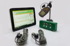
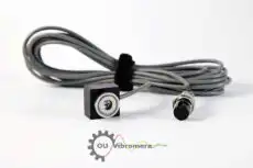
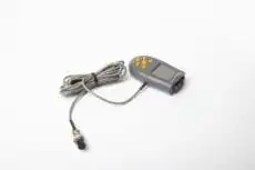
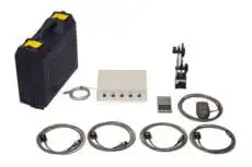
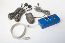
ਫੀਲਡ ਵਿੱਚ, ਉਹੀ ਯੰਤਰ ਜੋ ਸਪੈਕਟ੍ਰਾ ਕੈਪਚਰ ਕਰਦਾ ਹੈ, ਆਮ ਤੌਰ ’ਤੇ ਸਪੀਡ ਰੈਫਰੈਂਸ ਵੀ ਪ੍ਰਦਾਨ ਕਰਦਾ ਹੈ। ਇੱਕ ਪੋਰਟੇਬਲ ਦੋ-ਚੈਨਲ ਐਨਾਲਾਈਜ਼ਰ ਜਿਵੇਂ ਕਿ Balanset-1A, ਜੋ ਇਸਦੇ ਆਪਟੀਕਲ ਲੇਜ਼ਰ ਟੈਕੋਮੀਟਰ ਨਾਲ ਲੈਸ ਹੈ, ਜੋ ਇੱਕ ਪੱਟੀ ’ਤੇ ਟਰਿੱਗਰ ਕਰਦਾ ਹੈ ਪਰਾਵਰਤਕ ਟੇਪ, ਰਨ-ਅੱਪ ਜਾਂ ਕੋਸਟ-ਡਾਊਨ ਦੌਰਾਨ ਸਿੰਕ੍ਰੋਨਾਈਜ਼ਡ ਸਪੈਕਟ੍ਰਾ ਅਤੇ 1× ਐਂਪਲੀਟਿਊਡ-ਅਤੇ-ਫੇਜ਼ ਰਿਕਾਰਡ ਕਰਦਾ ਹੈ — ਉਹ ਕੱਚਾ ਮਟੀਰੀਅਲ ਜਿਸ ਤੋਂ ਇੱਕ ਕੈਸਕੇਡ ਡਾਇਗ੍ਰਾਮ ਬਣਾਇਆ ਜਾਂਦਾ ਹੈ। ਕਿਉਂਕਿ ਮਾਪ ਮਸ਼ੀਨ ਦੇ ਆਪਣੇ ਬੇਅਰਿੰਗਾਂ ਵਿੱਚ ਓਪਰੇਟਿੰਗ ਸਪੀਡ ’ਤੇ ਲਿਆ ਜਾਂਦਾ ਹੈ, ਨਤੀਜੇ ਵਾਲਾ ਪਲਾਟ ਰੋਟਰ ਦੇ ਅਸਲ ਇੰਸਟਾਲ ਕੀਤੇ ਵਿਵਹਾਰ ਨੂੰ ਦਰਸਾਉਂਦਾ ਹੈ।
5. ਸੰਬੰਧਿਤ ਰਨ-ਅੱਪ / ਕੋਸਟ-ਡਾਊਨ ਪਲਾਟ
ਉਹੀ ਟ੍ਰਾਂਜ਼ੀਐਂਟ ਡਾਟਾ ਸੈੱਟ ਕਈ ਪੂਰਕ ਡਿਸਪਲੇਅ ਨੂੰ ਫੀਡ ਕਰਦਾ ਹੈ, ਅਤੇ ਤਜਰਬੇਕਾਰ ਵਿਸ਼ਲੇਸ਼ਕ ਆਜ਼ਾਦੀ ਨਾਲ ਇਹਨਾਂ ਵਿਚਕਾਰ ਸਵਿੱਚ ਕਰਦੇ ਹਨ:
- ਬੋਡ ਪਲਾਟ (Bode Plot): ਸਪੀਡ ਦੇ ਵਿਰੁੱਧ ਕਾਰਟੀਸ਼ੀਅਨ ਧੁਰਿਆਂ ’ਤੇ ਪਲਾਟ ਕੀਤੇ ਇੱਕ ਸਿੰਗਲ ਆਰਡਰ ਦਾ ਐਂਪਲੀਟਿਊਡ ਅਤੇ ਫੇਜ਼ — ਇੱਕ ਪੀਕ ਦੀ ਸਹੀ RPM ਪੜ੍ਹਨ ਲਈ ਆਦਰਸ਼।
- ਨਾਈਕੁਇਸਟ ਪਲਾਟ: ਇੱਕ ਆਰਡਰ ਦੇ ਵੈਕਟਰ ਦਾ ਰੀਅਲ-ਬਨਾਮ-ਇਮੈਜਿਨਰੀ ਟਰੇਸ, ਜੋ ਹਰੇਕ ਕ੍ਰਿਟੀਕਲ ਸਪੀਡ ’ਤੇ ਇੱਕ ਲੂਪ ਬਣਾਉਂਦਾ ਹੈ।
- ਕੈਂਪਬੈੱਲ ਡਾਇਗ੍ਰਾਮ: ਇੱਕ ਸੰਬੰਧਿਤ ਫ੍ਰੀਕੁਐਂਸੀ-ਬਨਾਮ-ਸਪੀਡ ਮੈਪ ਜੋ ਦਖਲਅੰਦਾਜ਼ੀ ਦੀ ਭਵਿੱਖਬਾਣੀ ਕਰਨ ਲਈ ਆਰਡਰ ਲਾਈਨਾਂ ਨੂੰ ਕੁਦਰਤੀ-ਫ੍ਰੀਕੁਐਂਸੀ ਲਾਈਨਾਂ ’ਤੇ ਓਵਰਲੇਅ ਕਰਦਾ ਹੈ।
ਜਿੱਥੇ ਬੋਡ ਅਤੇ ਨਾਈਕਵਿਸਟ ਪਲਾਟ ਇੱਕ ਸਮੇਂ ’ਤੇ ਇੱਕ ਆਰਡਰ ’ਤੇ ਧਿਆਨ ਦਿੰਦੇ ਹਨ, ਵਾਟਰਫਾਲ ਪਲਾਟ ਪੂਰੇ ਪੂਰੀ ਸਪੈਕਟ੍ਰਮ ਨੂੰ ਹਰ ਸਪੀਡ ’ਤੇ ਦ੍ਰਿਸ਼ਟੀਗੋਚਰ ਰੱਖਦਾ ਹੈ। ਇਹ ਵਿਸਥਾਰ ਹੀ ਇਹ ਕਾਰਨ ਹੈ ਕਿ ਇਹ ਡੂੰਘਾਈ ਨਾਲ ਰੋਟਰਡਾਇਨਾਮਿਕ ਵਿਸ਼ਲੇਸ਼ਣ ਲਈ ਇੱਕ ਲਾਜ਼ਮੀ ਟੂਲ ਬਣਿਆ ਰਹਿੰਦਾ ਹੈ, ਜੋ ਮਸ਼ੀਨ ਦੇ ਪੂਰੇ ਓਪਰੇਟਿੰਗ ਰੇਂਜ ਵਿੱਚ ਇਸਦੇ ਵਿਵਹਾਰ ਦੀ ਇੱਕ ਪੂਰੀ ਤਸਵੀਰ ਦਿੰਦਾ ਹੈ।