కంపన విశ్లేషణలో షాఫ్ట్ Runoutని అర్థం చేసుకోవడం


Runout రోటర్లో లోపాలకు సాధారణ పదం, ఇవి షాఫ్ట్ చాలా నెమ్మదిగా తిరిగినప్పుడు కూడా ప్రతి విప్లవానికి ఒకసారి (1×) సంకేతాన్ని ఉత్పత్తి చేస్తాయి, అలాంటి సందర్భాలలో unbalance వంటి డైనమిక్ శక్తులు నిర్లక్ష్యం చేయదగినవి. కఠినంగా చెప్పాలంటే, ఇది షాఫ్ట్ యొక్క నిజమైన centreline. చాలా మంది విశ్లేషకులను ఇబ్బందిపెట్టే విషయం ఏమిటంటే runout పోలి ఉంటుంది exactly లో అసమతుల్యత వలె vibration డేటాతో — అయినప్పటికీ ఇది ద్రవ్యరాశి-సంబంధిత సమస్య కాదు మరియు దీనిని బ్యాలెన్సింగ్.
రెండు దృగ్విషయాలూ 1× వద్ద ఉంటాయి కాబట్టి running speed, వాటిని వేరు చేయడం రోటర్ డయాగ్నొస్టిక్స్లో మరింత ముఖ్యమైన నైపుణ్యాలలో ఒకటి. తప్పు చేస్తే ఎప్పటికీ కలవని బ్యాలెన్స్ను వెంటాడుతూ సమయం వృథా అవుతుంది; సరిగా చేస్తే అసలు లోపాన్ని సరిచేయడం లేదా బ్యాలెన్స్ ప్రయత్నించే ముందు దాన్ని శుభ్రంగా పరిహరించడం సాధ్యమవుతుంది. దిగువ విభాగాలు రెండు విభిన్న రకాల runoutలను నిర్వచిస్తాయి, అవి డయాగ్నొస్టిక్స్ను ఎందుకు భ్రష్టుపట్టిస్తాయో వివరిస్తాయి, మరియు వాటి ప్రభావాన్ని తొలగించడానికి ప్రమాణిక సాంకేతికతను వివరిస్తాయి.
1. Runout రకాలు: ఒక కీలకమైన వ్యత్యాసం
అన్నీ “runout” అనే ఒకే పదం అర్థించగల రెండు మూలభూతంగా భిన్నమైన విషయాలను వేరు చేయడంతో మొదలవుతాయి.
మెకానికల్ రన్అవుట్
మెకానికల్ runout అనేది షాఫ్ట్ యొక్క నిజమైన భౌతిక లేదా జ్యామితీయ లోపం షాఫ్ట్ యొక్క: ఉపరితలం పరిపూర్ణంగా గుండ్రంగా లేదు, లేదా ఇది భ్రమణ అక్షంపై పరిపూర్ణంగా కేంద్రీకృతంగా లేదు. సాధారణ కారణాలు ఇవి:
- Out-of-roundness: జర్నల్ మెషీనింగ్ వల్ల కొద్దిగా అండాకారంగా లేదా వేరే విధంగా తప్పు ఆకారంలో ఉంటుంది.
- Eccentricity: పుల్లీ, కప్లింగ్ లేదా గేర్ వంటి భాగం షాఫ్ట్ కేంద్రరేఖకు సంబంధించి కేంద్రం నుండి బయటగా మెషీన్ చేయబడి లేదా అమర్చబడి ఉంటుంది.
- వంగిన లేదా విరిగిన షాఫ్ట్: a permanent bend ప్రతి విప్లవంతో ఒక స్థిర బిందువు దాటి ఉపరితలాన్ని లోపలికి మరియు బయటకు సర్వే చేస్తుంది. సంబంధిత తాత్కాలిక వెర్షన్, thermal bow, యంత్రం వేడెక్కేటప్పుడు కనిపించి స్థిరపడే కొద్దీ అదృశ్యమవుతుంది.
ఇది నిజమైన జ్యామితీయ లక్షణం కాబట్టి, మెకానికల్ runoutను షాఫ్ట్ను చేతితో నెమ్మదిగా తిప్పుతున్నప్పుడు డయల్ ఇండికేటర్తో నేరుగా కొలవొచ్చు. మొత్తం ఇండికేటర్ రీడింగ్ తనిఖీ నివేదికలలో పేర్కొనబడిన విలువ, మరియు మా షాఫ్ట్ రేడియల్ రన్అవుట్ (TIR) కాలిక్యులేటర్ ఆ రీడింగ్ను అనుమతించదగిన సహనానికి సంబంధించడంలో సహాయపడుతుంది.
విద్యుత్ రన్అవుట్
ఎలక్ట్రికల్ runout అనేది షాఫ్ట్ ఆకారంలో లోపం కాదు, కానీ ఒక కొలత కళంకం నాన్-కాంటాక్ట్కు ప్రత్యేకమైన ఎడ్డీ-కరెంట్ ప్రాక్సిమిటీ ప్రోబులు. ఈ ప్రోబ్లు అధిక-పౌనఃపున్య అయస్కాంత క్షేత్రాన్ని నెలకొల్పి, షాఫ్ట్ ఉపరితలం దానిని ఎంతగా లోడ్ చేస్తుందో అనుసరించి అంతరాన్ని అంచనా వేస్తాయి. ఆ ఉపరితలంలో అయస్కాంత లేదా విద్యుత్ ధర్మాలలో స్థానికంగా వ్యత్యాసాలు ఉంటే, నిజమైన షాఫ్ట్-టు-ప్రోబ్ దూరం సంపూర్ణంగా స్థిరంగా ఉన్నప్పటికీ ప్రోబ్ హెచ్చుతగ్గులతో కూడిన అంతరాన్ని నివేదిస్తుంది. దీని కారణాలు జ్యామితీయమైనవి కాకుండా లోహశాస్త్ర మరియు ఉపరితల సంబంధమైనవి:
- పదార్థ పారగమ్యతలో వ్యత్యాసాలు: స్థానికంగా అయస్కాంతీకరించబడిన మచ్చ — తరచుగా జర్నల్పై మాగ్నెటిక్-బేస్ డయల్ ఇండికేటర్ను ఉంచినప్పటి అవశేషం — బలమైన, శాశ్వతమైన 1× సంకేతాన్ని ఉత్పత్తి చేస్తుంది.
- ఉపరితల ముగింపులో మార్పులు: ప్రోబ్’స్ వీక్షణ ప్రాంతంలో గీతలు, గుంటలు, లేదా పరికరపు గుర్తులు.
- అసమాన పదార్థ కూర్పు: షాఫ్ట్ యొక్క మిశ్రమం లేదా లోహశాస్త్ర నిర్మాణంలో వ్యత్యాసాలు.
అత్యంత కీలకంగా, విద్యుత్ రన్అవుట్ డయల్ ఇండికేటర్కు అదృశ్యంగా ఉంటుంది — జ్యామితి సరిగ్గా ఉంటుంది — అయినప్పటికీ ఇది టర్బోమెషినరీలో ఒక ప్రధాన లోపం మూలం, ఇక్కడ API 670వంటి ప్రమాణాల ప్రకారం పర్యవేక్షించబడుతున్నప్పుడు, ప్రాక్సిమిటీ ప్రోబ్లు ప్రాథమిక సెన్సార్లుగా ఉంటాయి.
2. రన్అవుట్ వ్యాధిస్థానం మరియు బ్యాలెన్సింగ్ను ఎందుకు దెబ్బతీస్తుంది
ఏ రకమైన రన్అవుట్ నుండి వచ్చే సంకేతం అయినా 1× నడుపు వేగంలో ఉంటుంది — అన్బ్యాలెన్స్ వలె సరిగ్గా అదే పౌనఃపున్యం — ఇది విశ్లేషకుడికి రెండు విభిన్న సమస్యలను సృష్టిస్తుంది.
- అది అసమతుల్యతగా మారువేషం వేసుకుంటుంది: లో ఒక పెద్ద 1× శిఖరం spectrum అన్బ్యాలెన్స్ అని నమ్మకంగా కానీ తప్పుగా నిర్ధారణ చేయడానికి పురికొల్పుతుంది, బ్యాలెన్సింగ్ ప్రయత్నాలను ప్రేరేపిస్తుంది, ఇవి అనవసరమైనవి మరియు సరిచేయడానికి అదనపు ద్రవ్యరాశి లేనందున విఫలమవడానికి నిర్ణయింపబడినవి.
- అది నిజమైన బ్యాలెన్సింగ్ను కలుషితం చేస్తుంది: నిజమైన అసమతుల్యత ఉన్నప్పుడు is ఉంటే, రన్అవుట్ వెక్టర్ దానికి జోడవుతుంది. రోటర్ను నిజాయితీగా బ్యాలెన్స్ చేయడానికి ఏ ప్రయత్నమైనా ముందుగా నిజమైన డైనమిక్ ప్రతిస్పందనను వేరుచేయాలి, అంటే రన్అవుట్ భాగాన్ని కొలవడం మరియు వెక్టోరియల్ వ్యవకలనం ద్వారా మొత్తం 1× సంకేతం నుండి దాన్ని తీసివేయడం.
అందువల్ల ఒక 1× శిఖరం మాత్రమే నిర్ధారణను స్థిరపరచదు — రన్అవుట్ వంటి సారూప్యతలకు వ్యతిరేకంగా నిజమైన అన్బ్యాలెన్స్ను ధృవీకరించడం, misalignment, a cracked rotor, or resonance సమర్థవంతమైన వైబ్రేషన్ విశ్లేషణ యొక్క హృదయం diagnosis.
3. రన్అవుట్ నష్టపరిహారం: స్లో-రోల్ వెక్టర్
ఆమోదయోగ్యమైన పరిష్కారం ఏమిటంటే రన్అవుట్ కాంపెన్సేషన్, ప్రాక్సిమిటీ ప్రోబ్లతో సాధనపరచబడిన ఏ యంత్రాన్నైనా విశ్లేషించడంలో ఒక అవసరమైన దశ. ఇది మూడు దశలలో సాగుతుంది:
- Slow roll: యంత్రాన్ని ఉద్దేశపూర్వకంగా తక్కువ వేగంలో నడుపుతారు — సాధారణంగా 200–500 rpm — ఇక్కడ అన్బ్యాలెన్స్ నుండి కేంద్రాపసారి శక్తులు నగణ్యంగా ఉంటాయి, కాబట్టి దాదాపు మొత్తం 1× సంకేతమూ రన్అవుట్ అవుతుంది.
- స్లో-రోల్ వెక్టర్ను కొలవడం: ఈ వేగంలో రికార్డ్ చేయబడిన 1× వైబ్రేషన్ వెక్టర్ (వ్యాప్తి మరియు phase) “స్లో-రోల్” లేదా “రన్అవుట్” వెక్టర్గా నమోదు చేయబడుతుంది.
- వెక్టర్ను తీసివేయడం: ఆ నిల్వ చేయబడిన స్లో-రోల్ వెక్టర్ అప్పుడు పూర్తి నిర్వహణ వేగంలో కొలవబడిన 1× వైబ్రేషన్ వెక్టర్ నుండి వెక్టర్గా తీసివేయబడుతుంది.
మిగిలేది ఏమిటంటే రన్అవుట్-పరిహారం చేయబడిన 1× వెక్టర్, అన్బ్యాలెన్స్ మరియు ఇతర రోటర్డైనమిక్ శక్తుల నుండి షాఫ్ట్ యొక్క నిజమైన డైనమిక్ చలనాన్ని సూచిస్తుంది. ఈ నష్టపరిహారం చేయబడిన విలువ — ముడి పఠనం కాదు — వ్యాధిస్థానాన్ని నడపాలి మరియు కరెక్షన్ వెయిట్లు.
4. క్షేత్రంలో కొలవడం మరియు నష్టపరిహారం
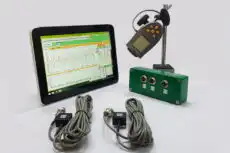
అదే సూత్రం పోర్టబుల్ పని వరకు వర్తిస్తుంది, యంత్రాలు ఉపయోగించినప్పటికీ accelerometers శాశ్వతంగా అమర్చిన ప్రోబ్లకు బదులుగా. ఒక చర్య తీసుకునే ముందు మంచి విధానం field balance అనేది ఏదైనా ట్రయల్ మాస్ జోడించే ముందు డయల్ ఇండికేటర్తో మెకానికల్ రన్అవుట్ను ధృవీకరించడం మరియు అవశేష అయస్కాంతత కోసం షాఫ్ట్ను పరీక్షించడం, సారూప్యతలను నిరాకరించడం. ఒక పోర్టబుల్ ద్వి-ఛానల్ విశ్లేషకుడు, ఉదాహరణకు Balanset-1A 1× వ్యాప్తి మరియు దశను కొలుస్తుంది, దానిపై బ్యాలెన్సింగ్ ఆధారపడుతుంది; మరియు యంత్రం అనుమతించినచోట స్లో-రోల్ సూచనను సంగ్రహించడం వల్ల విశ్లేషకుడు 1× స్పందన నిజంగా వేగంతో పెరుగుతుందా — ఇది నిజమైన అన్బ్యాలెన్స్ యొక్క లక్షణం — లేదా స్థిరంగా ఉంటుందా అని నిర్ధారించగలడు; స్థిరంగా ఉంటే అది నేరుగా రన్అవుట్కు సూచిస్తుంది.
