Application of the Fourier Transform to the Analysis of Vibration Signals
આન્દ્રે શેલ્કોવેન્કો. વિકાસકર્તાઓમાંના એક અને Vibromera ના સ્થાપક.
લેખના અનુવાદમાં અચોક્કસતા હોઈ શકે છે.
ફોરિયર ટ્રાન્સફોર્મ અને સિગ્નલ સ્પેક્ટ્રમ
In many cases the task of obtaining (calculating) the spectrum of a signal is as follows. There is an ADC, which with sampling frequency Fd transforms continuous signal, which comes to its input during time T, into digital samples – N pieces. Then this array of samples is fed to some program (for example ફોરિયરસ્કોપ) જે કેટલાક આંકડાકીય મૂલ્યો N/2 ને આઉટપુટ કરે છે.
પ્રોગ્રામ યોગ્ય રીતે કામ કરે છે કે કેમ તે ચકાસવા માટે, અમે બે sin(10*2*pi*x)+0.5*sin(5*2*pi*x) ના સરવાળા તરીકે નમૂનાઓની શ્રેણી બનાવીએ છીએ અને તેને પ્રોગ્રામમાં ફીડ કરીએ છીએ. પ્રોગ્રામ નીચે મુજબ દોર્યું:
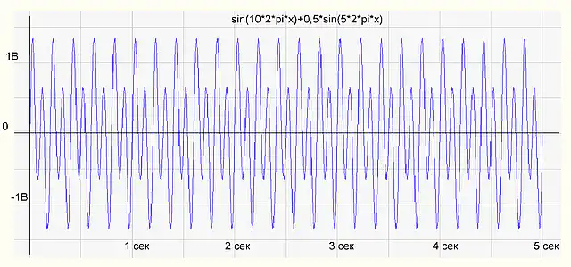
ફિગ.1 સિગ્નલના સમય કાર્યનો ગ્રાફ
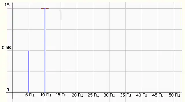
ફિગ.2 સિગ્નલ સ્પેક્ટ્રમનો ગ્રાફ
There are two harmonics on the spectrum graph – 5 Hz with amplitude of 0.5 V and 10 Hz with amplitude of 1 V, everything is as in the formula of the original signal. Everything is fine, the grogram works correctly.
આનો અર્થ એ છે કે જો આપણે બે સાઇનસૉઇડ્સના મિશ્રણમાંથી ADC ઇનપુટમાં વાસ્તવિક સિગ્નલ ફીડ કરીએ છીએ, તો અમને બે હાર્મોનિક્સનો સમાવેશ કરતું સમાન સ્પેક્ટ્રમ મળશે.
તેથી, અમારા વાસ્તવિક માપેલ સંકેત 5 સે. સમયગાળો, એડીસી દ્વારા ડિજિટાઇઝ્ડ, એટલે કે રજૂ સ્વતંત્ર દ્વારા નમૂનાઓ, એ છે સ્વતંત્ર બિન-સામયિક સ્પેક્ટ્રમ
ગાણિતિક દૃષ્ટિકોણથી - આ શબ્દસમૂહમાં કેટલી ભૂલો છે?
હવે એ જ સિગ્નલને 0.5 સેકન્ડ માટે માપવાનો પ્રયાસ કરીએ.
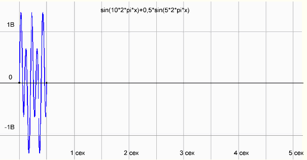
ફિગ.3 0.5 સેકન્ડના માપન સમયગાળા માટે ફંક્શન sin(10*2*pi*x)+0.5*sin(5*2*pi*x) નો ગ્રાફ
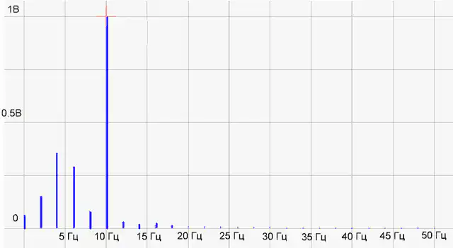
Fig.4 કાર્યનું સ્પેક્ટ્રમ
અહીં કંઈક ખોટું છે! 10 Hz પર હાર્મોનિક સામાન્ય રીતે દોરવામાં આવે છે, અને 5 Hz પર હાર્મોનિકને બદલે કેટલાક અસ્પષ્ટ હાર્મોનિક્સ છે.
ઇન્ટરનેટ પર તેઓ કહે છે કે નમૂનાના અંતમાં શૂન્ય ઉમેરવું જરૂરી છે અને સ્પેક્ટ્રમ સામાન્ય રીતે દોરવામાં આવશે.
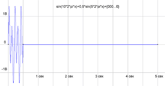
Fig.5 અમે નમૂનામાં 5 સેકન્ડ સુધી શૂન્ય ઉમેર્યા છે
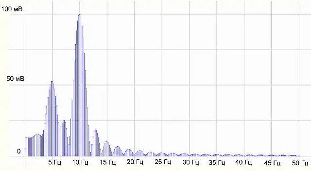
ફિગ.6. સ્પેક્ટ્રમ મેળવ્યું.
તે બિલકુલ નથી. મારે સિદ્ધાંત સાથે વ્યવહાર કરવો પડશે. પર જઈએ વિકિપીડિયા - જ્ઞાનનો સ્ત્રોત.
સતત કાર્ય અને તેની ફ્યુરિયર શ્રેણીનું પ્રતિનિધિત્વ
ગાણિતિક રીતે, T સેકન્ડની અવધિ સાથેનું અમારું સિગ્નલ અમુક ફંક્શન f(x) છે જે અંતરાલ {0, T} પર આપવામાં આવે છે (આ કિસ્સામાં X સમય છે). આવા ફંક્શનને હંમેશા ફોર્મના હાર્મોનિક ફંક્શન્સ (સાઇન અથવા કોસાઇન) ના સરવાળા તરીકે રજૂ કરી શકાય છે:

(1), જ્યાં:
k એ ત્રિકોણમિતિ કાર્યની સંખ્યા છે ( હાર્મોનિક ઘટકની સંખ્યા, હાર્મોનિકની સંખ્યા)
T - સેગમેન્ટ જ્યાં કાર્ય વ્યાખ્યાયિત થયેલ છે (સિગ્નલની અવધિ)
k-th હાર્મોનિક ઘટકનું કદ,
θk- kth હાર્મોનિક ઘટકનો પ્રારંભિક તબક્કો
"શ્રેણીના સરવાળા તરીકે કાર્યને રજૂ કરવાનો" તેનો અર્થ શું છે? તેનો અર્થ એ છે કે દરેક બિંદુ પર ફ્યુરિયર શ્રેણીના હાર્મોનિક ઘટકોના મૂલ્યો ઉમેરીને, આપણે તે બિંદુએ આપણા કાર્યનું મૂલ્ય મેળવીએ છીએ.
(વધુ કડક રીતે, ફંક્શન f(x) થી શ્રેણીનું સરેરાશ ચોરસ વિચલન શૂન્ય તરફ વલણ ધરાવે છે, પરંતુ સરેરાશ ચોરસ કન્વર્જન્સ હોવા છતાં, ફંક્શનની ફ્યુરિયર શ્રેણીને, સામાન્ય રીતે કહીએ તો, બિંદુએ બિંદુએ તેની સાથે કન્વર્જ થવાની જરૂર નથી.)
આ શ્રેણી ફોર્મમાં પણ લખી શકાય છે:
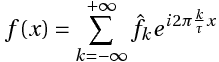
(2),
જ્યાં  , kth જટિલ કંપનવિસ્તાર.
અથવા

(3)
ગુણાંક (1) અને (3) વચ્ચેનો સંબંધ નીચેના સૂત્રો દ્વારા વ્યક્ત કરવામાં આવે છે:
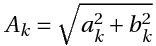
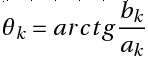
Note that all these three representations of Fourier series are perfectly equivalent. Sometimes when working with Fourier series, it is more convenient to use exponents of imaginary argument instead of sines and cosines, i.e. to use Fourier transform in complex form. But it is convenient for us to use formula (1), where the Fourier series is represented as a sum of cosines with corresponding amplitudes and phases. Strictly speaking, the Fourier transform of a real signal does produce complex coefficients (form (3)): each coefficient carries both the amplitude and the phase of its harmonic. For a real signal these complex coefficients possess conjugate (Hermitian) symmetry — the negative-frequency half simply mirrors the positive-frequency half and carries no extra information. That is why, from the complex coefficients, we can always pass to the real non-negative amplitudes Ak and phases θk of formula (1) — and it is exactly this amplitude spectrum that analysis programs plot.
નીચે લીટી:
સિગ્નલોના સ્પેક્ટ્રલ પૃથ્થકરણ માટેનો ગાણિતિક આધાર ફોરિયર ટ્રાન્સફોર્મ છે.
ફ્યુરિયર ટ્રાન્સફોર્મ ચોક્કસ કંપનવિસ્તાર અને તબક્કાઓ સાથે ત્રિકોણમિતિ વિધેયો (સાઇન અને/અથવા કોસાઇન) ની અનંત સંખ્યા (અનંત શ્રેણી) ના સરવાળા તરીકે અંતરાલ {0, T} પર વ્યાખ્યાયિત સતત ફંક્શન f(x) (સિગ્નલ) રજૂ કરવાની મંજૂરી આપે છે. અંતરાલ {0, T} પર પણ ગણવામાં આવે છે. આવી શ્રેણીને ફોરિયર શ્રેણી કહેવામાં આવે છે.
કેટલાક વધુ મુદ્દાઓ નોંધો, જેની સમજ સિગ્નલ વિશ્લેષણમાં ફોરિયર ટ્રાન્સફોર્મને યોગ્ય રીતે લાગુ કરવા માટે જરૂરી છે. જો આપણે સમગ્ર X-અક્ષ પર ફ્યુરિયર શ્રેણી (સાઇનસોઇડ્સનો સરવાળો) ધ્યાનમાં લઈશું તો આપણે જોઈશું કે અંતરાલ {0, T} ની બહાર ફ્યુરિયર શ્રેણીનું કાર્ય સમયાંતરે આપણા કાર્યનું પુનરાવર્તન કરશે.
ઉદાહરણ તરીકે, ફિગ. 7 માંના ગ્રાફમાં, મૂળ ફંક્શનને અંતરાલ {-T\2, +T\2} પર વ્યાખ્યાયિત કરવામાં આવ્યું છે, અને ફૌરિયર શ્રેણી સમગ્ર x-અક્ષ પર વ્યાખ્યાયિત સામયિક કાર્ય રજૂ કરે છે.
This is because the sinusoids themselves are periodic functions, so their sum will also be a periodic function.
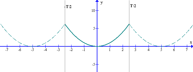
Figure 7 Representation of a non-periodic source function by a Fourier series
Thus:
Our original function is a continuous, non-periodic function defined on some segment of length T.
The spectrum of this function is discrete, i.e. it is represented as an infinite series of harmonic components – a Fourier series.
In fact, Fourier series defines some periodic function, which coincides with our function on the interval {0, T}, but for us this periodicity is not essential.
Next.
The periods of harmonic components are multiples of the interval {0, T}, on which the initial function f(x) is defined. In other words, the periods of harmonics are multiples of the duration of the signal measurement. For example, the period of the first harmonic in a Fourier series is equal to the interval T in which the function f(x) is defined. The period of the second harmonic in a Fourier series is equal to the interval T/2. And so on (see Figure 8).
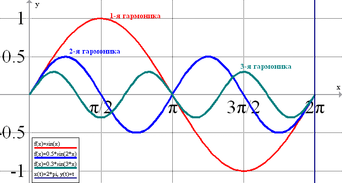
Fig. 8 Periods (frequencies) of harmonic components of the Fourier series (here T=2π)
Accordingly, the frequencies of harmonic components are multiples of 1/T. That is, frequencies of harmonic components Fk are Fk= k\T, where k runs values from 0 to ∞, for example, k=0 F0=0; k=1 F1=1\T; k=2 F2=2\T;k=3 F3=3\T;…. Fk= k\T (at zero frequency, a constant component).
Let our initial function, is a signal recorded during T=1 sec. Then the period of the first harmonic will be equal to the duration of our signal T1=T=1 sec and the frequency of the harmonic is equal to 1 Hz. The period of the second harmonic will be equal to the duration of our signal divided by 2 (T2=T/2=0.5 sec.) and the frequency is equal to 2 Hz. For the third harmonic, T3=T/3 sec and the frequency is 3 Hz. And so on.
The step between harmonics in this case is 1 Hz.
Thus, a signal with a duration of 1 sec can be decomposed into harmonic components (to obtain a spectrum) with a frequency resolution of 1 Hz.
To increase the resolution by a factor of 2 to 0.5 Hz, it is necessary to increase the duration of measurement by a factor of 2 to 2 sec. A 10-second signal can be decomposed into harmonic components (spectrum) with a frequency resolution of 0.1 Hz. There are no other ways to increase frequency resolution. You can explore this relationship with our FFT Resolution Calculator.
There is a way to artificially increase the signal duration by adding zeros to the array of samples. But it does not increase the real frequency resolution.
Discrete signals and discrete Fourier transform
With the development of digital technology the ways of measurement data (signals) storage have changed. Whereas previously a signal could be recorded on a tape recorder and stored on a tape in analog form, now signals are digitized and stored in files in computer memory as a set of numbers (counts).
The usual scheme of signal measurement and digitization looks as follows.
Measuring transducer —- Signal normalizer —- ADC —– Computer
(Fig.9 Schematic of the measuring channel)
The signal from the measuring transducer goes to the ADC for a period of time T. The signal readings (sampling) received during time T are transmitted to the computer and saved in the memory.
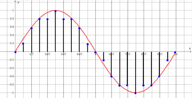
Fig.10 Digitized signal – N samples received for time T
What are the requirements to signal digitization parameters? A device which converts the input analog signal into a discrete code (digital signal) is called an analog-to-digital converter (ADC) (© Wiki).
One of the basic parameters of ADC is the maximum sampling rate – the frequency of sampling of a signal which is continuous in time. Sample rate is measured in hertz. ((© Wiki))
According to Kotelnikov’s theorem, if a continuous signal has a spectrum limited by the frequency Fmax, it can be fully and uniquely reconstructed from its discrete samples taken at time intervals Δt ≤ 1/(2*Fmax), ie with a sampling frequency Fd ≥ 2*Fmax, where Fd – sampling frequency; Fmax – the maximum frequency of the signal spectrum. In other words, the frequency of signal digitization (sampling frequency of ADC) must be at least twice the maximum frequency of the signal we want to measure.
And what will happen if we take samples with lower frequency than required by Kotelnikov’s theorem?
In this case there is an “aliasing” effect (aka stroboscopic effect, moiré effect), in which a high frequency signal after digitization turns into a low frequency signal, which in fact does not exist. In Fig. 11 the red sine wave of high frequency is the real signal. The blue sine wave of lower frequency is a fictitious signal, arising due to the fact that during the sampling time has time to pass more than half a period of the high-frequency signal.
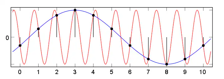
Fig. 11. Appearance of a spurious low frequency signal at an insufficiently high sampling rate
To avoid the aliasing effect, a special anti-alias filter (low-pass filter) is placed before the ADC. It passes frequencies lower than half of the ADC sampling frequency and cuts off higher frequencies.
In order to calculate signal spectrum by its discrete samples the discrete Fourier transform (DFT) is used. Note again that the spectrum of a discrete signal is “by definition” limited to a frequency Fmax smaller than half the sampling frequency Fd. Therefore, the spectrum of a discrete signal can be represented by the sum of a finite number of harmonics, in contrast to the infinite sum for the Fourier series of a continuous signal, whose spectrum can be unlimited. According to Kotelnikov’s theorem, the maximum frequency of a harmonic must be such that it accounts for at least two samples, so the number of harmonics is equal to half the number of samples of a discrete signal. That is, if there are N samples in the sample, the number of harmonics in the spectrum will be N/2.
Consider now the discrete Fourier transform (DFT).
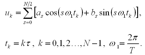
Comparing it with the Fourier series
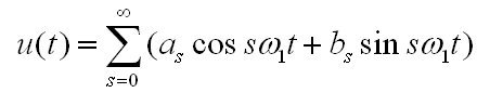
As we can see, they coincide, except for the fact that time in the FFT is discrete and the number of harmonics is limited to N/2, which is half the number of samples.
DFT formulas are written in dimensionless integer variables k, s, where k is the number of signal samples, s is the number of spectral components.
The value s shows the number of full harmonic oscillations per period T (signal measurement duration). The discrete Fourier transform is used to find the amplitudes and phases of harmonics numerically, i.e. “on the computer”.
As it was already said above, when decomposing a non-periodic function (our signal) into Fourier series, the resulting Fourier series actually corresponds to a periodic function with period T (Fig.12).
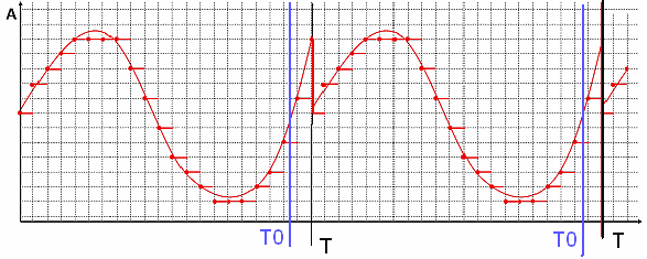
Fig.12. Periodic function f(x) with period T0, with period T>T0
As can be seen in Fig. 12, the function f(x) is periodic with period T0. However, due to the fact that the measuring sample length T is not equal to the function period T0, the function obtained as a Fourier series has a discontinuity at point T. As a result, the spectrum of this function will contain a large number of high-frequency harmonics. This phenomenon is known as spectral leakage, and in practice it is reduced by windowing the signal before the transform. If the duration of measuring sample T coincided with the period of function T0, then the spectrum obtained after the Fourier transform would contain only the first harmonic (a sinusoid with a period equal to the duration of the sample), because the function f(x) is a sinusoid.
In other words, the DFT program “does not know” that our signal is a “slice of a sine wave”, but tries to represent as a series a periodic function which has a discontinuity due to the discontinuity of separate pieces of the sine wave.
As a result, harmonics appear in the spectrum, which should, in total, represent the shape of the function, including this discontinuity.
Thus, to get a “correct” spectrum of a signal which is a sum of several sinusoids with different periods, it is necessary that an integer number of periods of each sinusoid should be present on the measuring period of the signal. In practice, this condition can be met with a sufficiently long duration of signal measurement.
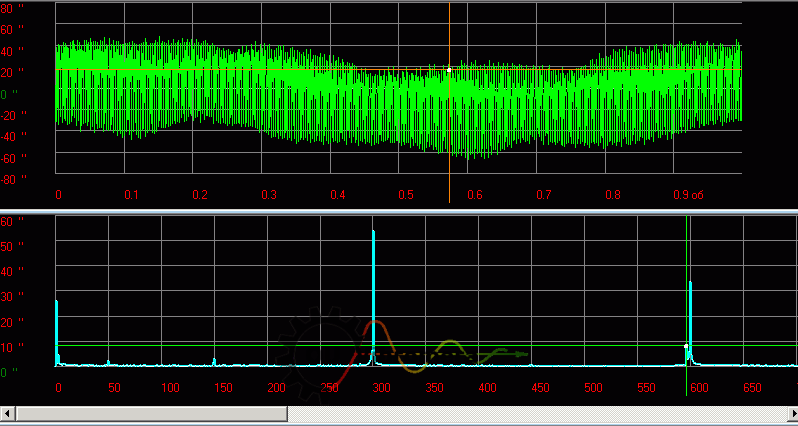
ફિગ.13 કાઇનેમેટિક એરર સિગ્નલ ફંક્શન અને ગિયરબોક્સના સ્પેક્ટ્રમનું ઉદાહરણ
At shorter duration the picture will look “worse”:
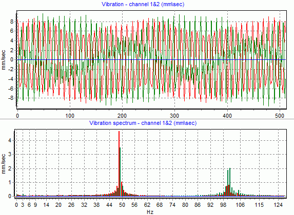
Fig.14 Example of rotor vibration function and spectrum
In practice, it can be difficult to understand where the “real components” and where the “artifacts” caused by inconsistency of component periods and signal sampling durations or “jumps and breaks” in the waveform. Of course, the words “real components” and “artifacts” are put in quotes for a reason. The presence of many harmonics on the spectrum graph does not mean that our signal actually consists of them. It is like thinking that number 7 “consists” of numbers 3 and 4. The number 7 can be thought of as the sum of 3 and 4 – that is correct.
So also our signal… or rather not even “our signal”, but a periodic function composed by repeating our signal (sample) can be represented as a sum of harmonics (sine waves) with certain amplitudes and phases. But in many cases important for practice (see figures above) it is indeed possible to relate the harmonics obtained in the spectrum also to real processes having cyclic character and contributing significantly to the form of the signal.
Some results
1. A real measured signal with T sec. duration digitized by ADC, i.e. represented by a set of discrete samples (N pieces), has a discrete non-periodic spectrum represented by a set of harmonics (N/2 pieces).
2. The signal is represented by a set of real values. Its DFT spectrum is a set of complex coefficients with conjugate symmetry; from them the amplitude spectrum is obtained — a set of real non-negative amplitudes (and phases) at positive frequencies, and it is this one-sided amplitude spectrum that is plotted in practice. The two-sided complex form with negative frequencies and the one-sided amplitude/phase form are equivalent representations of the same spectrum — for signal analysis it is usually more convenient to work with the one-sided amplitude spectrum.
3. T ના સમયે માપવામાં આવેલ સિગ્નલ માત્ર T સમયે જ નક્કી થાય છે. આપણે સિગ્નલને માપવાનું શરૂ કરતા પહેલા શું થયું અને તે પછી શું થશે તે વિજ્ઞાનને ખબર નથી. અને અમારા કિસ્સામાં તે રસપ્રદ નથી. સમય-મર્યાદિત સિગ્નલનું FFT તેનું "વાસ્તવિક" સ્પેક્ટ્રમ આપે છે, તે અર્થમાં કે અમુક પરિસ્થિતિઓમાં તે તેના ઘટકોના કંપનવિસ્તાર અને આવર્તનની ગણતરી કરવાની મંજૂરી આપે છે.