坎貝爾圖
一種頻率對轉速的圖表,揭示旋轉機械中的臨界轉速、陀螺效應分裂與共振危險區——從微型渦輪機到多兆瓦壓縮機組。




定義
A 坎貝爾圖 (亦稱為 進動轉速圖 或 干擾圖)是一種繪製 自然頻率 轉子-軸承系統在垂直軸上,對水平軸上的旋轉速度繪圖。疊加對角線的激振階次線(1×、2×、3×…);無論激振線與自然頻率曲線在哪裡相交,都會產生 臨界轉速 存在。此圖表是判斷機器運行範圍是否安全地遠離 共振 條件的圖表。
簡言之:坎貝爾圖回答了一個問題—— 「此轉子會在哪些速度下共振,且這些速度與我計畫運轉的速度有多接近?」
歷史背景
Wilfred Campbell 於 1924 年在通用電氣研究汽輪機盤的周向波時發表了此概念。他最初的圖表繪製了盤的振動模態對轉速的關係,以預測運轉期間破壞性共振出現的位置。
此方法填補了自 1890 年代以來困擾工程師的空白。W. J. M. Rankine 於 1869 年的軸進動分析錯誤預測超臨界運轉不可能。Gustaf de Laval 於 1889 年透過在第一個臨界速度之上運轉汽輪機證明了相反結論。Henry Jeffcott 於 1919 年發表的里程碑論文最終解釋了 為何 超臨界運轉是穩定的,但坎貝爾圖為工程師提供了 視覺化工具 以精確預測這些危險轉速的位置——以及如何設計避開它們。
在隨後的幾十年中,此概念從盤振動擴展至完整的橫向轉子分析、扭振分析,甚至聲學。如今,所有主要的 API、ISO 與 IEC 旋轉機械標準皆要求或建議進行坎貝爾圖分析。
圖表結構解析
坎貝爾圖在單一圖表中包含四類資訊。正確判讀交點前,必須理解每一層資訊。
座標軸
橫軸為轉速,通常以 RPM 或 Hz 表示。縱軸為頻率,以 Hz 或 CPM 表示。當兩軸使用相同單位時,1× 激振線恰好呈 45°——這是驗證比例尺是否正確的有效視覺檢查方法。
自然頻率曲線
每條曲線代表轉子-軸承-支撐系統的一個振動模式。在最簡單的情況下(剛性軸承、無陀螺效應),這些曲線為水平線,因為自然頻率不隨速度改變。實際上,陀螺力矩與速度相關的軸承剛性會導致曲線傾斜、分裂或兩者兼具。
模式依撓曲形狀標記:第一彎曲(一個反節點)、第二彎曲(兩個反節點與一個節點)、第三彎曲等。若相關,亦可繪製扭轉與軸向模式。
正向與反向進動
當陀螺效應顯著時,每個非旋轉狀態下的自然頻率會隨著轉速增加分裂為兩條曲線:
- 正向進動(FW): 模態進動方向與軸旋轉方向相同。陀螺剛化效應使其頻率 返回頂部.
- 反向進動(BW): 模態進動方向與旋轉方向相反。陀螺軟化效應使其頻率 降低.
正向進動模態是 不平衡 驅動共振的主要關注點,因為不平衡會激勵同步正向進動。
激振階次線
這些是從原點發射的直線對角線。每條線代表一個激振,其頻率為轉速的固定倍數:
| 線 | 關係 | 典型來源 |
|---|---|---|
| 1× | f = 1 × RPM/60 | 質量不平衡,轉子彎曲 |
| 2× | f = 2 × RPM/60 | 不對心,軸裂紋、橢圓度 |
| 3×、4×… | f = n × RPM/60 | 齒輪嚙合、葉輪/葉片通過、聯軸器缺陷 |
| 0.43–0.48× | f ≈ 0.45 × RPM/60 | 液膜軸承中的油膜渦動 |
| 葉片通過頻率 | f = Z × RPM/60 | 葉片數 Z × 運轉速度 |
交點 = 臨界轉速
激振線與自然頻率曲線之間的每個交點都標示了一個潛在的共振點。該交點處的 RPM 值即為該特定模態-激振組合的臨界轉速。如果運轉範圍包含或接近該 RPM,機器就有產生高振動幅值的風險。
互動式坎貝爾圖
下方的 SVG 顯示了一個雙軸承、柔性軸轉子的典型坎貝爾圖。將游標懸停在元素上以識別模態、激振線和臨界轉速交點。
如何閱讀與解讀坎貝爾圖
逐步解讀程序
識別運轉速度範圍
找到標示最小和最大連續運轉速度的垂直帶或刻度線。在圖 1 中,此範圍為 9,000–12,000 RPM。
首先追蹤 1× 線
1× 同步線最為關鍵,因為不平衡(存在於每個轉子中)會在 1× 運轉速度下產生激振。找出它與順向進動曲線交叉的每個點。
讀取交點的水平座標
每個交點的 x 座標即為臨界速度。記錄每個臨界速度及其涉及的模態編號。
檢查 2× 及更高階的交點
對 2×、3×、葉片通過頻率及次同步線重複此步驟。這些交點是次要臨界轉速——能量低於 1×,但仍可能引起振動問題,特別是當激振源強烈時。
計算分離裕度
對於每個臨界轉速,計算其到運轉範圍最近邊緣的百分比距離。並與適用的標準 (API 617, API 612, ISO, OEM 規格) 進行比較。
評估曲線斜率
陡峭向上傾斜的順向進動 (FW) 曲線表示強烈的陀螺效應——常見於懸臂轉子。近乎平坦的曲線則表示系統由軸承剛性主導。
識別危險區域
如果兩個臨界轉速夾住運轉範圍且裕度不足,則必須修改設計:軸承剛性、軸直徑、支撐剛性或運轉速度必須改變。
⚠️ 常見的誤解: 逆向進動模態很少對不平衡激振產生響應,因為不平衡僅產生順向進動。與逆向進動 (BW) 曲線的交點通常不是真正的運轉臨界轉速——它們被包含在圖中是為了完整性,以及存在其他激振源的情況(例如密封中的反向流動)。
理解分離裕度
安全運轉要求運轉速度範圍必須遠離每個臨界轉速,以便共振放大在可容忍範圍內。所需的裕度取決於共振峰的尖銳程度,由 放大係數 (AF).
- 低 AF (< 2.5)表示強阻尼——轉子可在臨界速度附近甚至於臨界速度運轉,而不會產生過大振動。
- 高 AF (> 8) 意味著尖銳的峰值——即使與臨界轉速偏離幾個百分點,也會導致危險的幅值增長。
典型的工業實踐要求 15–30% 的分離裕度,但具體要求取決於適用標準和 AF 值。
陀螺效應與頻率分裂
當旋轉盤進動(晃動)時,會產生耦合兩個垂直平面運動的陀螺力矩。這種耦合將零轉速時的單一自然頻率分裂為任何非零轉速下的兩個不同頻率。
物理原理
具有陀螺效應的轉子運動方程形式如下:
其中 M 是質量矩陣, C 阻尼矩陣, G 斜對稱陀螺矩陣(與轉速 Ω 成正比),以及 K 剛性矩陣。由於 G 取決於轉速,特徵值——因此自然頻率——會隨 Ω 變化。
何者決定分裂幅度?
極慣性矩 (Ip) 與徑向慣性矩 (Id) 的比值控制著陀螺效應的強度。盤狀元件 (Ip/Id > 1) 產生強烈的分裂。細長軸段 (Ip/Id ≈ 0) 產生的分裂可忽略不計。
懸臂轉子(單級泵葉輪、渦輪增壓器輪、懸臂式砂輪)展現最顯著的陀螺分裂。在此類設計中,正向進動的第一臨界速度可能比零速自然頻率高出 20–40%,意味著坎貝爾圖與簡單的「平直線」模型截然不同。對懸臂轉子進行平直線分析會低估第一 FW 臨界速度並高估第一 BW 臨界速度,可能導致錯誤的運轉速度決策。
軸承類型如何影響坎貝爾圖形狀
軸承將轉子連接到定子,並定義決定自然頻率的邊界條件。不同的軸承技術會產生根本不同的圖形形狀。
| 軸承類型 | 剛性行為 | 對坎貝爾曲線的影響 | 其他注意事項 |
|---|---|---|---|
| 滾動軸承 (球軸承、滾子軸承) | 隨轉速幾乎保持恆定 | 自然頻率曲線大致平坦(水平),除非陀螺效應佔主導地位 | 缺陷頻率 (BPFO、BPFI、BSF) 會在非整數階次增加激振線 |
| 液膜(軸頸) | 剛性與阻尼隨轉速增加(索默費爾德數變化) | 曲線向上傾斜的陡峭程度超過僅由陀螺效應產生的程度 | 交叉耦合剛性可能導致不穩定(油膜渦動/油膜振盪);增加 0.43–0.48× 次同步線 |
| 傾斜瓦滑動軸承 | 剛性隨轉速增加;交叉耦合極小 | 與普通滑動軸承斜率相似,但穩定性更佳 | 依 API 617 標準,為高速壓縮機首選 |
| 主動磁浮軸承 | 透過控制演算法可程式化;可為恆定、增加或適應性 | 曲線可刻意塑形,將臨界速度移離運轉範圍 | 控制迴路頻寬限制高頻率下可達到的最大剛性 |
| 氣體軸承(箔片/氣靜壓) | 剛性隨轉速急劇增加;阻尼極低 | 曲線急劇上升;高 Q 值共振 | 低阻尼使分離裕度更為關鍵 |
各向異性支撐
當軸承支撐座或基礎在水平與垂直方向具有不同剛性時,每個模態會進一步分裂為水平與垂直變體。坎貝爾圖則會顯示更多曲線——每個模態包含水平前向進動、垂直前向進動、水平後向進動與垂直後向進動。這在具有柔性基礎的水平機器中很常見。
API 617 與分離裕度要求
對於石油、化學與氣體服務中的離心與軸流壓縮機,API 標準 617(第 8 版,2014 年;第 9 版,2022 年)強制要求進行嚴格的坎貝爾圖分析,作為橫向轉子動力學研究的一部分。
API 617 分離裕度公式
其中 SM 為所需分離裕度 (%),而 AF 為該臨界速度下不平衡響應(波特)圖的放大係數。
| AF 值 | 依公式之 SM | 解讀 |
|---|---|---|
| < 2.5 | 無需 SM | 臨界阻尼;可在臨界速度下運轉 |
| 3.5 | 8.5% | 中等阻尼;小裕度即可 |
| 5.0 | 12.1% | 典型用於傾斜瓦軸承 |
| 8.0 | 14.4% | 尖銳峰值;需要較大裕度 |
| 12.0 | 15.4% | 非常尖銳;接近 16% 上限 |
| > ~11 | ≤ 16%(上限) | API 將低於最低轉速的臨界轉速 SM 上限設為 16% |
將此應用於坎貝爾圖
在設計審查期間,工程師從坎貝爾圖讀取每個臨界轉速,然後檢查波德圖中對應的 AF。如果 SMactual ≥ SM所需,則設計通過。否則,工程師必須修改軸承、軸幾何形狀或運轉範圍,直到滿足所有裕度要求。
其他具有類似要求的標準: API 612(汽輪機)、API 613(齒輪箱)、API 672(成套空氣壓縮機)、ISO 10814(臨界轉速接近度公差)、ISO 22266(往復式機械的機械振動)。每個標準使用略有不同的公式或固定百分比閾值,但都依賴坎貝爾圖作為原始資料。
建立坎貝爾圖:分析與實驗
分析(有限元分析 / 轉移矩陣)方法
建立轉子模型
將軸、盤、葉輪、聯軸器和襯套離散化為樑單元(Timoshenko 或 Euler-Bernoulli)或 3D 實體/殼單元。包含質量、剛性和陀螺項。
定義軸承特性
輸入與轉速相關的剛性和阻尼係數(每個液膜軸承 8 個係數:Kxx,Kxy,Kyx,Kyy,Cxx,Cxy,Cyx,Cyy)。對於滾動軸承,使用恆定剛性值。
設定轉速範圍和增量
定義從 0 到至少最大連續轉速 115% 的轉速掃描(根據 API 617 跳脫轉速要求),並使用足夠細的 RPM 增量(通常為 100–500 RPM 步進)以準確捕捉曲線形狀。
求解複數特徵值問題
在每個轉速步進,求解 det(K + iΩG − ω²M) = 0 以找到自然頻率 ωn (虛部)和阻尼(實部)。虛部成為坎貝爾圖上的 y 座標。
繪製並疊加激振線
繪製所有模態與轉速的關係,添加 1×、2× 和其他相關激振線,並標記交點。
實驗方法(來自現場資料)
當機器已存在時,可以從升速或惰轉降速過程中的振動測量中提取坎貝爾圖:
- 在軸承位置安裝加速規或近接探棒。
- 在緩慢啟動(或跳脫後惰轉降速)期間連續記錄振動。
- 生成 瀑布(級聯)圖:在連續 RPM 值下拍攝的 FFT 頻譜堆疊。
- 識別每個 RPM 切片中的頻率峰值——這些是由主導階次激發的自然頻率。
- 繪製峰值頻率與 RPM 的關係以產生實驗坎貝爾圖。
惰轉降速測試通常比啟動產生更清晰的資料,因為機器平順減速,沒有馬達啟動時的扭矩波動。從跳脫轉速到靜止進行惰轉降速,並進行連續高解析度資料採集(≥ 4,096 條線,0.5 秒平均)。如果機器使用變頻器,請編程 50–100 RPM/秒的線性斜坡以獲得最佳頻率解析度。
依機器類型分類之應用
| 機器 | 典型轉速範圍 | 坎貝爾圖關鍵關注點 | governing 標準 |
|---|---|---|---|
| 離心壓縮機 | 3,000–60,000 RPM | 多個臨界轉速;液膜軸承不穩定;密封交叉耦合;通常跳脫轉速以下有 2–4 個模態 | API 617 |
| 汽輪機 | 3,000–15,000 RPM | 葉片通過激振;暖機期間熱彎曲改變模態;高階次的盤模態 | API 612 |
| 燃氣渦輪機 | 3,600–30,000 RPM | 雙轉軸設計需為每個轉軸分別繪製坎貝爾圖;擠壓膜阻尼器效應 | API 616 / OEM |
| 電動機 / 發電機 | 750–36,000 RPM | 2× 電源頻率的電磁激振;VFD 驅動馬達需掃過共振區 | API 541 / IEC 60034 |
| 泵 | 1,000–12,000 RPM | 懸臂葉輪具有強烈的陀螺效應;葉片通過激振;耐磨環剛性隨時間變化 | API 610 |
| 機床主軸 | 5,000–60,000+ RPM | 預壓角接觸軸承;高轉速下預壓損失導致頻率軟化 | ISO 15641 / OEM |
| 渦輪增壓器 | 30,000–300,000 RPM | 浮動環軸承具有複雜的內/外油膜動力學;次同步渦動常見 | OEM / SAE |
| 風力渦輪機變速箱 | 10–20 RPM(轉子);高達 1,800 RPM(高速軸) | 用於齒輪嚙合共振的扭轉坎貝爾圖;多種速比 | IEC 61400 / AGMA |
設計階段用途
在設計階段,坎貝爾圖指導關於軸徑、軸承位置、軸承類型以及葉輪/盤幾何形狀的決策。將臨界轉速移動僅 10% 可能需要將軸承跨距改變 50 mm 或軸徑改變 5 mm —— 該圖表向工程師精確顯示所需的偏移量。
故障排除用途
若機器在特定速度下產生高 1× 振動,坎貝爾圖可快速顯示該速度是否與預測的臨界速度重合。若重合,解決方案為改變運轉速度、增加阻尼(例如擠壓膜阻尼器)或提升動平衡校正品質。若不重合,高振動可能另有根本原因,如機械鬆動或軸承缺陷。
運轉指導
坎貝爾圖定義了 禁止轉速範圍 —— 由於臨界轉速落在該帶域內而不允許持續運轉的 RPM 帶域。變速機(VFD 驅動壓縮機、負載跟隨的渦輪發電機組)必須審查其坎貝爾圖,以確保沒有連續運轉工況點位於禁止帶域內。在啟動或停機期間瞬態通過臨界轉速是可以接受的,前提是加速度足夠高以防止振幅累積。
測量圖表預測的內容
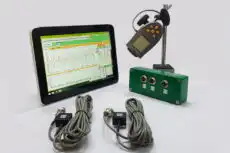
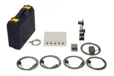
Balanset-1A 便攜式分析儀記錄您進行實驗坎貝爾圖所需的振動資料 —— 升速和惰轉降速期間的頻譜與 RPM 關係。現場雙平面動平衡校正。售價 €1,975 起。
相關圖表與曲線圖
坎貝爾圖是轉子動力學分析中幾個相互關聯的視覺化工具之一。每個工具都有獨特的用途。
坎貝爾圖
座標軸: 自然頻率與轉速。
顯示: 臨界轉速 將 發生位置(預測性)。基於特徵值分析或從瀑布圖資料中提取。
波德圖
座標軸: 振動振幅與相位對旋轉速度。
顯示: 實際升速/惰轉降速期間的測量響應。確認臨界轉速位置並提供用於裕度計算的放大係數。
瀑布圖(級聯圖)
座標軸: 頻譜與轉速(3D)。
顯示: 每個 RPM 步進下的完整頻譜內容。提取實驗坎貝爾圖的原始資料。同時揭示所有激振階次。
無阻尼臨界轉速圖
座標軸: 自然頻率與軸承剛性(非轉速)。
顯示: 臨界轉速如何隨支撐剛性變化而偏移。用於早期設計,在生成完整坎貝爾圖之前確定軸承剛性範圍。
軌跡圖
座標軸: 單一轉速下的 X 位移與 Y 位移。
顯示: 特定 RPM 下軸運動的形狀。前向渦動產生圓形軌跡;後向渦動產生逆行橢圓。
穩定性圖
座標軸: 對數減縮量(或實特徵值)與轉速。
顯示: 系統穩定(正阻尼)與不穩定(負阻尼)的區域。坎貝爾圖擴展一個維度。
實務案例:高速壓縮機
考慮一台設計用於 15,000 RPM 連續運轉(250 Hz)的離心壓縮機,跳脫轉速為 17,250 RPM(115%)。
坎貝爾圖結果
- 第1階 FW 臨界(1×): 5,200 RPM(86.7 Hz)——安全地低於運行範圍。
- 第2 FW臨界(1×): 19,800 RPM(330 Hz)— 高於跳機轉速。
- 第1 FW × 2×: 2,600轉/分——僅在啟動過程中出現,會快速通過。
裕度檢查
最低運行轉速:12,000 RPM。與第一階前向渦動臨界轉速(5,200 RPM)的錯頻裕度:
由波德圖得出此臨界轉速的 AF 為 4.2,依 API 617 公式所需 SM 為 10.7%。實際 SM 為 56.7%,遠超要求 — 無問題。
與第二階前向渦動臨界轉速(19,800 RPM)至跳機轉速(17,250 RPM)之間的錯頻裕度:
該臨界轉速的AF為6.5,要求SM需達13.6%。實際SM為14.8%,勉強通過。工程師在報告中標註此項,並建議在車間機械運轉試驗期間覆核精確的AF值。
如果積垢使葉輪質量增加3%,第二階前進渦動(FW)臨界轉速會從19,800降至約19,200轉/分,將裕度降至11.3%——低於所要求的13.6%。這種情境必須在隨API資料表一併提交的敏感度分析中加以呈現。
坎貝爾圖軟體工具
坎貝爾圖可由通用有限元素分析(FEA)平台與專用轉子動力學軟體產生。
| 工具 | 類型 | 備註 |
|---|---|---|
| ANSYS Mechanical(轉子動力學) | 通用有限元素分析 | 完整的3D實體加樑元素模型;內建坎貝爾圖後處理器;需搭配RGYRO進行阻尼模態分析 |
| Siemens Simcenter 3D | 通用有限元素分析 | 適用於多轉子系統的超級元件縮減;內建軌跡圖與穩定性圖 |
| DyRoBeS | 專用轉子動力學 | 基於樑元素;運算快速;依API 684教學指南,廣泛應用於壓縮機與渦輪機原廠(OEM) |
| XLTRC²(德州農工大學) | 專用轉子動力學 | 以試算表為基礎的工作流程;強大的軸承係數庫;廣泛用於泵與壓縮機分析 |
| MADYN 2000 | 專用轉子動力學 | 德國研發;有限元加傳遞矩陣混合演算法;非常適合扭轉加橫向耦合分析 |
| COMSOL Multiphysics | 通用有限元素分析 | 適用於自訂模型的轉子動力學模組;可編程後處理 |
| Bently Nevada System 1 / ADRE | 狀態監測 | 從現場振動資料提取實驗性坎貝爾圖;即時追蹤 |
使用坎貝爾圖(Campbell Diagram)時常見的錯誤
1. 忽略陀螺效應
執行無阻尼、零轉速的模態分析,並假設所得頻率即為臨界轉速。這樣做會得出平直線,完全忽略正進動/逆進動的分裂現象。務必求解與轉速相關的特徵值問題。
2. 使用過於粗略的轉速增量
如果在轉速達10,000轉/分的機器上,測試步階為2,000轉/分,您可能會完全錯過某個狹窄的交叉點。建議使用100–500轉/分的增量,以確保曲線定義的可靠性。
3. 混淆坎貝爾圖與波德圖
坎貝爾圖用於預測 其中 臨界轉速的位置;波德圖則顯示 有多嚴重 確實如此。依照API 617,完整的轉子動力學評估需要同時具備兩者。
4. 忽略基礎與支撐的柔性
採用剛性支撐的轉子模型所得出的臨界轉速,會與同一轉子架設在實際柔性基礎上的結果不同。應在模型中納入軸承座與基礎的柔度。
5. 忽略溫度與負載效應
軸承間隙會隨溫度變化,進而改變剛度係數。製程氣體密度會影響密封的交叉耦合效應。坎貝爾圖(Campbell diagram)應在最小與最大間隙/密度條件下分別繪製。
6. 將所有交點視為同等危險
1×與第一階前向模態相交,遠比4×與高階後向模態相交更為危險。應依激振能量與模態類型來排定優先順序。
需要現場振動數據?
Balanset-1A 在升速/惰轉降速期間擷取振動頻譜,用於瀑布圖與實驗坎貝爾圖。雙通道、雙平面,符合 ISO 1940 標準。透過 DHL Express / UPS 全球運送。
常見問題
坎貝爾圖與波德圖有何差異?
坎貝爾圖繪製系統自然頻率對旋轉速度——它預測 在哪些轉速下 存在臨界狀態。波德圖(Bode plot)則是將實際測得(或計算得出)的振動振幅與相位對轉速作圖——它顯示的是 振幅多大 轉子會在這些臨界轉速下產生振動。工程師使用坎貝爾圖(Campbell diagram)進行設計,並使用波德圖(Bode plot)進行驗證。API 617 壓縮機認證均要求提供這兩者。
API 617 要求臨界轉速的避讓裕度為何?
API 617採用公式SM = 17 × {1 − [1/(AF − 1.5)]},其中AF為該臨界轉速下的放大係數。若AF < 2.5, no margin is required because the resonance is overdamped. For typical tilting-pad bearings (AF = 4–8), required margins range from 10% to 15%. The maximum required SM is capped at 16% for critical speeds below minimum operating speed. For critical speeds above maximum continuous speed, the same formula applies but the margin is calculated as a percentage of the maximum continuous speed.
為什麼自然頻率會在坎貝爾圖上分裂為前進渦動與後退渦動?
旋轉盤件產生的陀螺力矩將轉子在兩個垂直平面上的運動耦合。此耦合產生兩種不同的進動模式:正向進動(與軸旋轉方向相同,因陀螺效應而剛性增加)與反向進動(與旋轉方向相反,因陀螺效應而剛性降低)。盤件的極慣量與徑向慣量比越高,分裂越強烈。在零速時無陀螺力矩,因此兩種模式合併為單一頻率。
能否從現場量測建立坎貝爾圖?
是的。可在連續啟動(或停機降速)過程中,使用加速度計或安裝於軸承座上的電渦流探頭記錄振動。將時域資料處理成瀑布圖(層疊圖)——即每個轉速增量下的一系列FFT頻譜。提取每個轉速步階的峰值頻率,再將這些峰值對轉速作圖,結果即為實驗性的坎貝爾圖(Campbell diagram)。停機降速通常能得到較乾淨的資料,因為不存在馬達啟動時的轉矩暫態。建議將降速率控制在50–100 RPM/s,並使用至少4,096條FFT譜線以獲得良好的頻率解析度。
坎貝爾圖應包含哪些激振階次?
至少務必納入 1× 線(不平衡——所有旋轉機械中最常見的單一激振來源)。加入 2× 以涵蓋不對中、軸橢圓度或軸裂紋。對於渦輪機械,應納入葉片通過頻率(葉片數 × 1×)與導葉通過頻率。對於齒輪系統,應納入齒輪嚙合頻率。對於採用油膜軸承的機器,加入 0.43–0.48× 線以涵蓋油膜渦動。若機器有已知的故障模式(例如具 6 爪的聯軸器),則應納入該階次(6×)。
軸承類型如何影響坎貝爾圖的形狀?
滾動軸承在整個轉速範圍內的剛性幾乎維持恆定,因此固有頻率曲線幾乎呈水平(平坦)狀態——唯一的斜率來自陀螺效應。油膜(軸頸)軸承則隨轉速升高,因油膜變薄而變得更硬,使固有頻率曲線上升得更陡峭。可傾瓦軸頸軸承的行為類似,但產生的交叉耦合較少,有助於提升轉子穩定性。主動磁浮軸承則可透過程式即時改變剛性,讓工程師能動態調整坎貝爾圖的形狀,以避開共振。