ანდრეი შელკოვენკო. Vibromera-ს ერთ-ერთი შემქმნელი და დამფუძნებელი.
სტატიის თარგმანი შეიძლება შეიცავდეს უზუსტობებს.
- ფურიეს ტრანსფორმაცია და სიგნალის სპექტრი
ხშირ შემთხვევაში სიგნალის სპექტრის მიღების (გამოანგარიშების) ამოცანა შემდეგია. არსებობს ADC, რომელიც შერჩევის სიხშირით Fd გარდაქმნის უწყვეტ სიგნალს, რომელიც მის შეყვანაში მოდის T დროში, ციფრულ ნიმუშებად - N ცალი. შემდეგ ნიმუშების ეს მასივი მიეწოდება რომელიმე პროგრამას (მაგალითად FourierScope) რომელიც გამოაქვს N/2 ზოგიერთი რიცხვითი მნიშვნელობები.
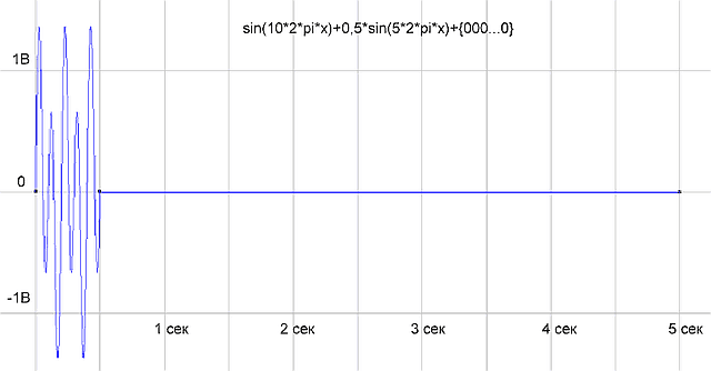
იმისათვის, რომ შევამოწმოთ, მუშაობს თუ არა პროგრამა სწორად, ჩვენ ვქმნით ნიმუშების მასივს ორი sin(10*2*pi*x)+0.5*sin(5*2*pi*x) ჯამის სახით და ვაწვდით მას პროგრამაში. პროგრამა ასახავდა შემდეგს:
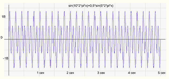
ნახ.1 სიგნალის დროის ფუნქციის გრაფიკი
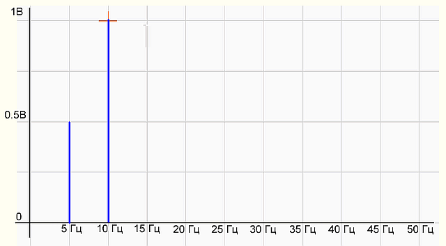
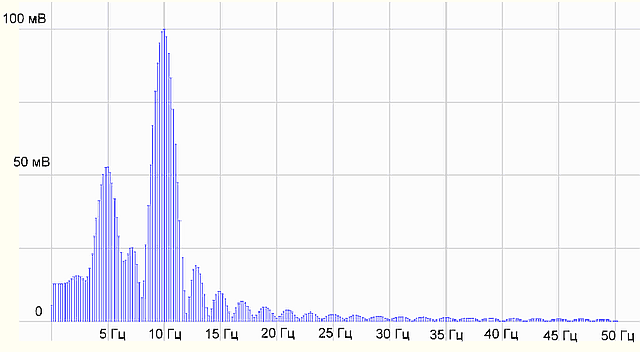
ნახ.2 სიგნალის სპექტრის გრაფიკი
სპექტრის გრაფიკზე ორი ჰარმონიაა - 5 ჰც ამპლიტუდით 0,5 ვ და 10 ჰც 1 ვ ამპლიტუდით, ყველაფერი ისეა, როგორც ორიგინალური სიგნალის ფორმულაში. ყველაფერი კარგადაა, გროგრამი მუშაობს გამართულად.
ეს ნიშნავს, რომ თუ ჩვენ მივაწვდით რეალურ სიგნალს ორი სინუსოიდის ნარევიდან ADC შეყვანაში, მივიღებთ მსგავს სპექტრს, რომელიც შედგება ორი ჰარმონიისგან.
ასე რომ, ჩვენი რეალური გაზომილი სიგნალი 5 წმ. ხანგრძლივობა, გაციფრული ADC-ით, ანუ წარმოდგენილი დისკრეტული გზით ნიმუშები, აქვს ა დისკრეტული არაპერიოდული სპექტრი.
მათემატიკური თვალსაზრისით - რამდენი შეცდომაა ამ ფრაზაში?
ახლა შევეცადოთ გავზომოთ იგივე სიგნალი 0,5 წამის განმავლობაში.
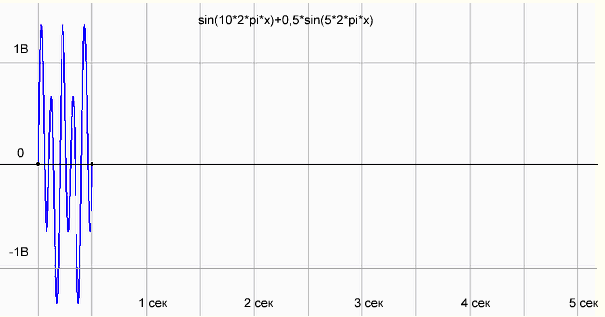
სურ.3 sin(10*2*pi*x)+0.5*sin(5*2*pi*x) ფუნქციის გრაფიკი 0.5 წმ.
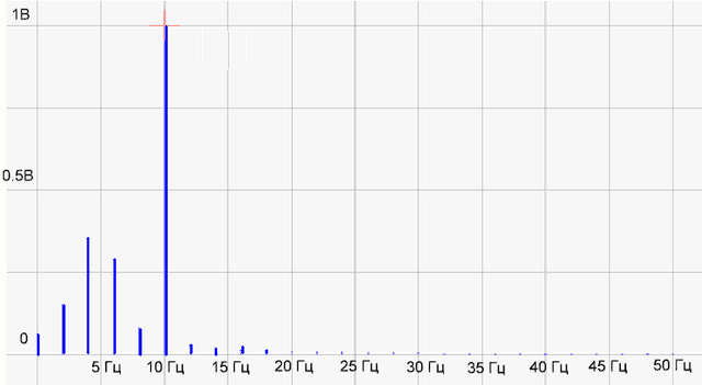
ნახ.4 ფუნქციის სპექტრი
აქ რაღაც არასწორია! 10 ჰც-ზე ჰარმონია ჩვეულებრივ შედგენილია, ხოლო 5 ჰც-ზე ჰარმონიის ნაცვლად არის გაურკვეველი ჰარმონია.
ინტერნეტში ამბობენ, რომ ნიმუშის ბოლოში ნულების დამატებაა საჭირო და სპექტრი ნორმალურად დაიხაზება.
ნახ.5 ნიმუშს დავამატეთ ნულები 5 წმ-მდე
სურ.6. მიღებული სპექტრი.
ეს სულაც არ არის. თეორიასთან მომიწევს საქმე. Წავიდეთ ვიკიპედია - ცოდნის წყარო.
2. უწყვეტი ფუნქცია და მისი ფურიეს რიგის წარმოდგენა
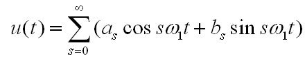
მათემატიკურად, ჩვენი სიგნალი T წამის ხანგრძლივობით არის გარკვეული ფუნქცია f(x) მოცემული ინტერვალზე {0, T} (ამ შემთხვევაში X არის დრო). ასეთი ფუნქცია ყოველთვის შეიძლება იყოს წარმოდგენილი ფორმის ჰარმონიული ფუნქციების ჯამი (სინუსი ან კოსინუსი):
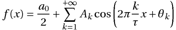
(1), სადაც:
k არის ტრიგონომეტრიული ფუნქციის რიცხვი (ჰარმონიული კომპონენტის რაოდენობა, ჰარმონიის რაოდენობა)
T - სეგმენტი, სადაც ფუნქცია განისაზღვრება (სიგნალის ხანგრძლივობა)
k-ე ჰარმონიული კომპონენტის აკ-ამპლიტუდა,
θk- kth ჰარმონიული კომპონენტის საწყისი ფაზა
რას ნიშნავს „ფუნქციის სერიის ჯამის სახით წარმოდგენა“? ეს ნიშნავს, რომ ფურიეს სერიის ჰარმონიული კომპონენტების მნიშვნელობების დამატებით თითოეულ წერტილში, ჩვენ ვიღებთ ჩვენი ფუნქციის მნიშვნელობას ამ წერტილში.
(უფრო მკაცრად, სერიის საშუალო კვადრატული გადახრა f(x) ფუნქციიდან ნულისკენ მიისწრაფვის, მაგრამ მიუხედავად საშუალო კვადრატული კონვერგენციისა, ფუნქციის ფურიეს სერიები, ზოგადად რომ ვთქვათ, არ არის საჭირო, რომ მას წერტილი-პუნქტი ემთხვეოდეს.)
ეს სერია ასევე შეიძლება დაიწეროს ფორმით:
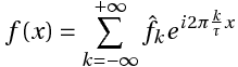
(2),
სადაც ![]() , kth რთული ამპლიტუდა.
, kth რთული ამპლიტუდა.
ან
(3)
(1) და (3) კოეფიციენტებს შორის კავშირი გამოიხატება შემდეგი ფორმულებით:
![]()
გაითვალისწინეთ, რომ ფურიეს სერიის სამივე წარმოდგენა სავსებით ექვივალენტურია. ზოგჯერ ფურიეს სერიებთან მუშაობისას უფრო მოსახერხებელია სინუსებისა და კოსინუსების ნაცვლად წარმოსახვითი არგუმენტების ექსპონენტების გამოყენება, ანუ რთული ფორმით ფურიეს ტრანსფორმაციის გამოყენება. მაგრამ ჩვენთვის მოსახერხებელია გამოვიყენოთ ფორმულა (1), სადაც ფურიეს რიგი წარმოდგენილია როგორც კოსინუსების ჯამი შესაბამისი ამპლიტუდებითა და ფაზებით. ნებისმიერ შემთხვევაში, არასწორია იმის თქმა, რომ რეალური სიგნალის ფურიეს გარდაქმნის შედეგი იქნება რთული ჰარმონიული ამპლიტუდები. როგორც Wiki სწორად ამბობს, „ფურიეს ტრანსფორმაცია (ℱ) არის ოპერაცია, რომელიც ასახავს რეალური ცვლადის ერთ ფუნქციას სხვა ფუნქციასთან, ასევე რეალური ცვლადის ფუნქციაზე“.
ქვედა ხაზი:
სიგნალების სპექტრული ანალიზის მათემატიკური საფუძველია ფურიეს ტრანსფორმაცია.
ფურიეს ტრანსფორმაცია საშუალებას გაძლევთ წარმოადგინოთ უწყვეტი ფუნქცია f(x) (სიგნალი), რომელიც განსაზღვრულია {0, T} ინტერვალზე, როგორც ტრიგონომეტრიული ფუნქციების (სინუსი და/ან კოსინუსი) უსასრულო რაოდენობის (უსასრულო სერიების) ჯამი გარკვეული ამპლიტუდებითა და ფაზებით. ასევე გათვალისწინებულია {0, T} ინტერვალზე. ასეთ სერიას ფურიეს სერია ეწოდება.
გაითვალისწინეთ კიდევ რამდენიმე პუნქტი, რომელთა გაგებაც საჭიროა სიგნალის ანალიზში ფურიეს ტრანსფორმაციის სწორი გამოყენებისთვის. თუ განვიხილავთ ფურიეს სერიას (სინუსოიდების ჯამს) მთელ X ღერძზე, დავინახავთ, რომ ინტერვალის გარეთ {0, T} ფურიეს სერიის ფუნქცია პერიოდულად გაიმეორებს ჩვენს ფუნქციას.
მაგალითად, ნახ. 7-ის გრაფიკზე თავდაპირველი ფუნქცია განსაზღვრულია ინტერვალზე {-T\2, +T\2}, ხოლო ფურიეს სერია წარმოადგენს პერიოდულ ფუნქციას, რომელიც განსაზღვრულია მთელ x ღერძზე.
This is because the sinusoids themselves are periodic functions, so their sum will also be a periodic function.
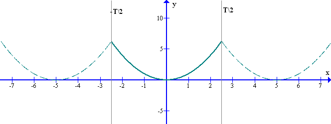
Figure 7 Representation of a non-periodic source function by a Fourier series
Thus:
Our original function is a continuous, non-periodic function defined on some segment of length T.
The spectrum of this function is discrete, i.e. it is represented as an infinite series of harmonic components – a Fourier series.
In fact, Fourier series defines some periodic function, which coincides with our function on the interval {0, T}, but for us this periodicity is not essential.
Next.
The periods of harmonic components are multiples of the interval {0, T}, on which the initial function f(x) is defined. In other words, the periods of harmonics are multiples of the duration of the signal measurement. For example, the period of the first harmonic in a Fourier series is equal to the interval T in which the function f(x) is defined. The period of the second harmonic in a Fourier series is equal to the interval T/2. And so on (see Figure 8).
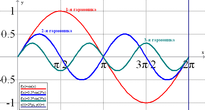
Fig. 8 Periods (frequencies) of harmonic components of the Fourier series (here T=2π)
Accordingly, the frequencies of harmonic components are multiples of 1/T. That is, frequencies of harmonic components Fk are Fk= k\T, where k runs values from 0 to ∞, for example, k=0 F0=0; k=1 F1=1\T; k=2 F2=2\T;k=3 F3=3\T;…. Fk= k\T (at zero frequency, a constant component).
Let our initial function, is a signal recorded during T=1 sec. Then the period of the first harmonic will be equal to the duration of our signal T1=T=1 sec and the frequency of the harmonic is equal to 1 Hz. The period of the second harmonic will be equal to the duration of our signal divided by 2 (T2=T/2=0.5 sec.) and the frequency is equal to 2 Hz. For the third harmonic, T3=T/3 sec and the frequency is 3 Hz. And so on.
The step between harmonics in this case is 1 Hz.
Thus, a signal with a duration of 1 sec can be decomposed into harmonic components (to obtain a spectrum) with a frequency resolution of 1 Hz.
To increase the resolution by a factor of 2 to 0.5 Hz, it is necessary to increase the duration of measurement by a factor of 2 to 2 sec. A 10-second signal can be decomposed into harmonic components (spectrum) with a frequency resolution of 0.1 Hz. There are no other ways to increase frequency resolution.
There is a way to artificially increase the signal duration by adding zeros to the array of samples. But it does not increase the real frequency resolution.
3. Discrete signals and discrete Fourier transform
With the development of digital technology the ways of measurement data (signals) storage have changed. Whereas previously a signal could be recorded on a tape recorder and stored on a tape in analog form, now signals are digitized and stored in files in computer memory as a set of numbers (counts).
The usual scheme of signal measurement and digitization looks as follows.
Measuring transducer —- Signal normalizer —- ADC —– Computer
(Fig.9 Schematic of the measuring channel)
The signal from the measuring transducer goes to the ADC for a period of time T. The signal readings (sampling) received during time T are transmitted to the computer and saved in the memory.
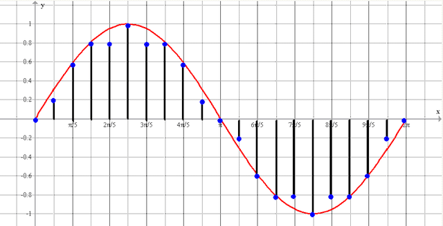
Fig.10 Digitized signal – N samples received for time T
What are the requirements to signal digitization parameters? A device which converts the input analog signal into a discrete code (digital signal) is called an analog-to-digital converter (ADC) (© Wiki).
One of the basic parameters of ADC is the maximum sampling rate – the frequency of sampling of a signal which is continuous in time. Sample rate is measured in hertz. ((© Wiki))
According to Kotelnikov’s theorem, if a continuous signal has a spectrum limited by the frequency Fmax, it can be fully and uniquely reconstructed from its discrete samples taken at time intervals T = 1/2*Fmax, ie with a frequency Fd ≥ 2*Fmax, where Fd – sampling frequency; Fmax – the maximum frequency of the signal spectrum. In other words, the frequency of signal digitization (sampling frequency of ADC) must be at least 2 times higher than the maximum frequency of the signal we want to measure.
And what will happen if we take samples with lower frequency than required by Kotelnikov’s theorem?
In this case there is an “aliasing” effect (aka stroboscopic effect, moiré effect), in which a high frequency signal after digitization turns into a low frequency signal, which in fact does not exist. In Fig. 11 the red sine wave of high frequency is the real signal. The blue sine wave of lower frequency is a fictitious signal, arising due to the fact that during the sampling time has time to pass more than half a period of the high-frequency signal.
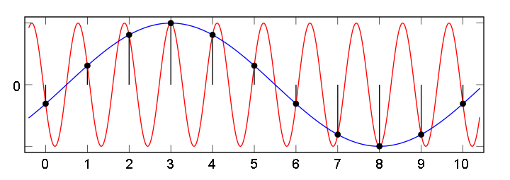
Fig. 11. Appearance of a spurious low frequency signal at an insufficiently high sampling rate
To avoid the aliasing effect, a special anti-alias filter (low-pass filter) is placed before the ADC. It passes frequencies lower than half of the ADC sampling frequency and cuts off higher frequencies.
In order to calculate signal spectrum by its discrete samples the discrete Fourier transform (DFT) is used. Note again that the spectrum of a discrete signal is “by definition” limited to a frequency Fmax smaller than half the sampling frequency Fd. Therefore, the spectrum of a discrete signal can be represented by the sum of a finite number of harmonics, in contrast to the infinite sum for the Fourier series of a continuous signal, whose spectrum can be unlimited. According to Kotelnikov’s theorem, the maximum frequency of a harmonic must be such that it accounts for at least two samples, so the number of harmonics is equal to half the number of samples of a discrete signal. That is, if there are N samples in the sample, the number of harmonics in the spectrum will be N/2.
Consider now the discrete Fourier transform (DFT).
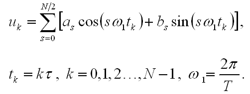
Comparing it with the Fourier series
As we can see, they coincide, except for the fact that time in the FFT is discrete and the number of harmonics is limited to N/2, which is half the number of samples.
DFT formulas are written in dimensionless integer variables k, s, where k is the number of signal samples, s is the number of spectral components.
The value s shows the number of full harmonic oscillations per period T (signal measurement duration). The discrete Fourier transform is used to find the amplitudes and phases of harmonics numerically, i.e. “on the computer”.
As it was already said above, when decomposing a non-periodic function (our signal) into Fourier series, the resulting Fourier series actually corresponds to a periodic function with period T (Fig.12).
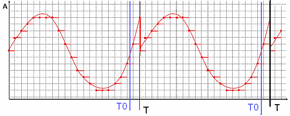
Fig.12. Periodic function f(x) with period T0, with period T>T0
As can be seen in Fig. 12, the function f(x) is periodic with period T0. However, due to the fact that the measuring sample length T is not equal to the function period T0, the function obtained as a Fourier series has a discontinuity at point T. As a result, the spectrum of this function will contain a large number of high-frequency harmonics. If the duration of measuring sample T coincided with the period of function T0, then the spectrum obtained after the Fourier transform would contain only the first harmonic (a sinusoid with a period equal to the duration of the sample), because the function f(x) is a sinusoid.
In other words, the DFT program “does not know” that our signal is a “slice of a sine wave”, but tries to represent as a series a periodic function which has a discontinuity due to the discontinuity of separate pieces of the sine wave.
As a result, harmonics appear in the spectrum, which should, in total, represent the shape of the function, including this discontinuity.
Thus, to get a “correct” spectrum of a signal which is a sum of several sinusoids with different periods, it is necessary that an integer number of periods of each sinusoid should be present on the measuring period of the signal. In practice, this condition can be met with a sufficiently long duration of signal measurement.
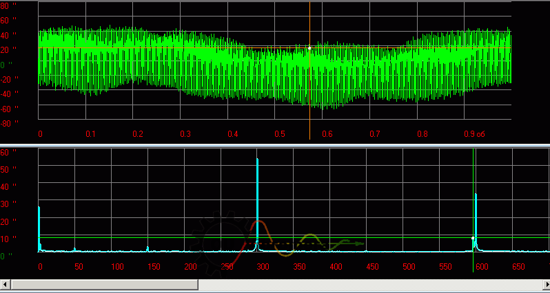
ნახ.13 გადაცემათა კოლოფის კინემატიკური შეცდომის სიგნალის ფუნქციისა და სპექტრის მაგალითი
At shorter duration the picture will look “worse”:
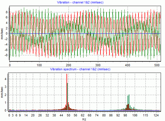
Fig.14 Example of rotor vibration function and spectrum
In practice, it can be difficult to understand where the “real components” and where the “artifacts” caused by inconsistency of component periods and signal sampling durations or “jumps and breaks” in the waveform. Of course, the words “real components” and “artifacts” are put in quotes for a reason. The presence of many harmonics on the spectrum graph does not mean that our signal actually consists of them. It is like thinking that number 7 “consists” of numbers 3 and 4. The number 7 can be thought of as the sum of 3 and 4 – that is correct.
So also our signal… or rather not even “our signal”, but a periodic function composed by repeating our signal (sample) can be represented as a sum of harmonics (sine waves) with certain amplitudes and phases. But in many cases important for practice (see figures above) it is indeed possible to relate the harmonics obtained in the spectrum also to real processes having cyclic character and contributing significantly to the form of the signal.
Some results
1. A real measured signal with T sec. duration digitized by ADC, i.e. represented by a set of discrete samples (N pieces), has a discrete non-periodic spectrum represented by a set of harmonics (N/2 pieces).
2. სიგნალი წარმოდგენილია მოქმედი მნიშვნელობების სიმრავლით და მისი სპექტრი წარმოდგენილია მოქმედი მნიშვნელობებით. ჰარმონიის სიხშირეები დადებითია. მხოლოდ იმიტომ, რომ მათემატიკურად უფრო მოსახერხებელია სპექტრის კომპლექსური ფორმით წარმოდგენა უარყოფითი სიხშირეების გამოყენებით, არ ნიშნავს იმას, რომ „ეს სწორია“ და „ასე უნდა გააკეთოთ ყოველთვის“.
3. T დროზე გაზომილი სიგნალი განისაზღვრება მხოლოდ T დროს. რა მოხდა მანამ, სანამ დავიწყებდით სიგნალის გაზომვას და რა მოხდება ამის შემდეგ, მეცნიერებისთვის უცნობია. და ჩვენს შემთხვევაში ეს არ არის საინტერესო. დროში შეზღუდული სიგნალის FFT იძლევა მის "რეალურ" სპექტრს, იმ გაგებით, რომ გარკვეულ პირობებში ის საშუალებას გაძლევთ გამოთვალოთ მისი კომპონენტების ამპლიტუდა და სიხშირე.
