Andrei Shelkovenko. Salah seorang pembangun dan pengasas Vibromera.
Terjemahan artikel mungkin mengandungi ketidaktepatan.
- Transformasi Fourier dan spektrum isyarat
Dalam banyak kes, tugas untuk mendapatkan (mengira) spektrum isyarat adalah seperti berikut. Terdapat ADC, yang dengan frekuensi pensampelan Fd mengubah isyarat berterusan, yang datang ke inputnya semasa T, ke dalam sampel digital - kepingan N. Kemudian pelbagai sampel ini disalurkan kepada beberapa program (contohnya FourierScope) yang mengeluarkan N/2 beberapa nilai berangka.
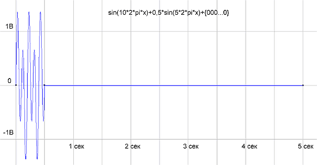
Untuk menyemak sama ada atur cara berfungsi dengan betul, kami membentuk tatasusunan sampel sebagai jumlah dua sin(10*2*pi*x)+0.5*sin(5*2*pi*x) dan suapkannya ke dalam atur cara. Program ini menarik perkara berikut:
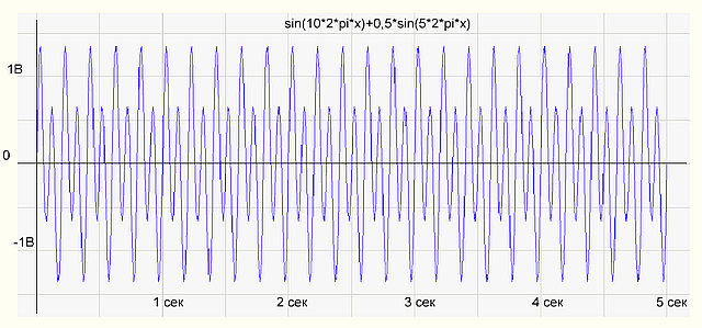
Rajah.1 Graf fungsi masa bagi isyarat
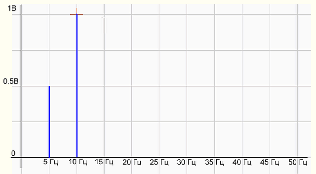
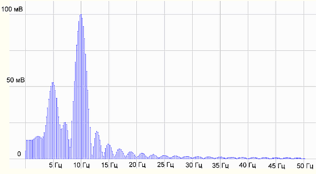
Rajah.2 Graf spektrum isyarat
Terdapat dua harmonik pada graf spektrum - 5 Hz dengan amplitud 0.5 V dan 10 Hz dengan amplitud 1 V, semuanya adalah seperti dalam formula isyarat asal. Semuanya baik-baik saja, grogram berfungsi dengan betul.
Ini bermakna jika kita memberi isyarat sebenar daripada campuran dua sinusoid ke input ADC, kita akan mendapat spektrum yang serupa yang terdiri daripada dua harmonik.
Jadi, kami sebenar isyarat yang diukur daripada 5 saat. tempoh masa, didigitalkan oleh ADC, iaitu diwakili secara diskret sampel, mempunyai a diskret tidak berkala spektrum.
Dari sudut pandangan matematik - berapa banyak kesilapan dalam frasa ini?
Sekarang mari kita cuba mengukur isyarat yang sama selama 0.5 saat.
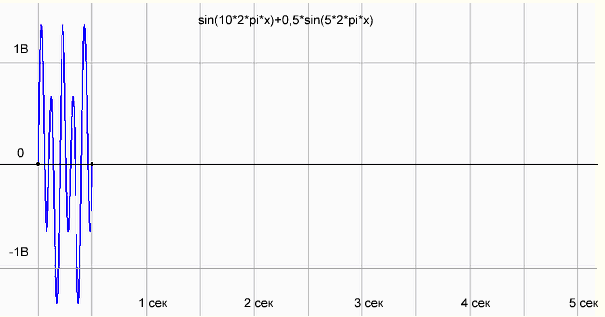
Rajah.3 Graf bagi fungsi sin(10*2*pi*x)+0.5*sin(5*2*pi*x) untuk tempoh pengukuran 0.5 saat
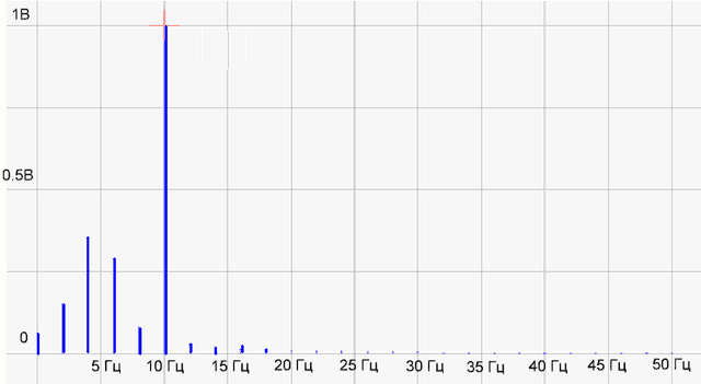
Rajah 4 Spektrum fungsi
Ada yang tidak kena di sini! Harmonik pada 10 Hz dilukis secara normal, dan bukannya harmonik pada 5 Hz terdapat beberapa harmonik yang tidak jelas.
Di Internet mereka mengatakan bahawa adalah perlu untuk menambah sifar pada penghujung sampel dan spektrum akan dilukis secara normal.
Rajah 5 Kami telah menambah sifar kepada sampel sehingga 5 saat
Rajah.6. Spektrum diperolehi.
Bukan itu sahaja. Saya perlu berurusan dengan teori. Mari pergi ke wikipedia - sumber ilmu.
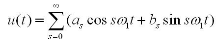
2. Fungsi berterusan dan perwakilan siri Fouriernya
Secara matematik, isyarat kami dengan tempoh T saat ialah beberapa fungsi f(x) yang diberikan pada selang {0, T} (X dalam kes ini ialah masa). Fungsi sedemikian sentiasa boleh diwakili sebagai jumlah fungsi harmonik (sinus atau kosinus) dalam bentuk:
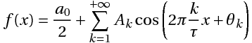
(1), di mana:
k ialah bilangan fungsi trigonometri ( bilangan komponen harmonik, bilangan harmonik)
T – segmen di mana fungsi ditentukan (tempoh isyarat)
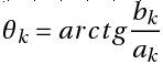
Ak- amplitud komponen harmonik ke-k,
θk- fasa awal komponen harmonik kth
Apakah yang dimaksudkan untuk "mewakili fungsi sebagai jumlah siri"? Ini bermakna dengan menambah nilai komponen harmonik siri Fourier pada setiap titik, kita mendapat nilai fungsi kita pada ketika itu.
(Lebih tegas lagi, sisihan purata kuasa dua siri daripada fungsi f(x) akan cenderung kepada sifar, tetapi walaupun terdapat penumpuan kuasa dua purata, siri Fourier bagi suatu fungsi tidak perlu, secara amnya, menumpu kepadanya titik demi titik. )
Siri ini juga boleh ditulis dalam bentuk:
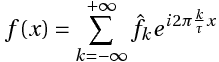
(2),
di mana ![]() , amplitud kompleks kth.
, amplitud kompleks kth.
atau
(3)
Hubungan antara pekali (1) dan (3) dinyatakan dengan formula berikut:
![]()
Ambil perhatian bahawa ketiga-tiga perwakilan siri Fourier ini adalah setara dengan sempurna. Kadangkala apabila bekerja dengan siri Fourier, adalah lebih mudah untuk menggunakan eksponen hujah khayalan dan bukannya sinus dan kosinus, iaitu menggunakan transformasi Fourier dalam bentuk kompleks. Tetapi adalah mudah untuk kita menggunakan formula (1), di mana siri Fourier diwakili sebagai jumlah kosinus dengan amplitud dan fasa yang sepadan. Walau apa pun, adalah salah untuk mengatakan bahawa hasil transformasi Fourier bagi isyarat sebenar akan menjadi amplitud harmonik yang kompleks. Seperti yang dinyatakan Wiki dengan betul, "Transformasi Fourier (ℱ) ialah operasi yang memetakan satu fungsi pembolehubah sebenar kepada fungsi lain juga pembolehubah sebenar."
Pokoknya:
Asas matematik untuk analisis spektrum isyarat ialah transformasi Fourier.
Transformasi Fourier membolehkan untuk mewakili fungsi berterusan f(x) (isyarat) yang ditakrifkan pada selang {0, T} sebagai jumlah nombor tak terhingga (siri tak terhingga) fungsi trigonometri (sinus dan/atau kosinus) dengan amplitud dan fasa yang pasti juga dipertimbangkan pada selang {0, T}. Siri sedemikian dipanggil siri Fourier.
Perhatikan beberapa perkara lagi, pemahaman yang diperlukan untuk aplikasi yang betul bagi transformasi Fourier kepada analisis isyarat. Jika kita menganggap siri Fourier (jumlah sinusoid) pada keseluruhan paksi X kita akan melihat bahawa di luar selang {0, T} fungsi siri Fourier akan mengulangi fungsi kita secara berkala.
Sebagai contoh, dalam graf dalam Rajah 7, fungsi asal ditakrifkan pada selang {-T\2, +T\2}, dan siri Fourier mewakili fungsi berkala yang ditakrifkan pada keseluruhan paksi-x.
This is because the sinusoids themselves are periodic functions, so their sum will also be a periodic function.
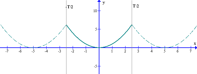
Figure 7 Representation of a non-periodic source function by a Fourier series
Thus:
Our original function is a continuous, non-periodic function defined on some segment of length T.
The spectrum of this function is discrete, i.e. it is represented as an infinite series of harmonic components – a Fourier series.
In fact, Fourier series defines some periodic function, which coincides with our function on the interval {0, T}, but for us this periodicity is not essential.
Next.
The periods of harmonic components are multiples of the interval {0, T}, on which the initial function f(x) is defined. In other words, the periods of harmonics are multiples of the duration of the signal measurement. For example, the period of the first harmonic in a Fourier series is equal to the interval T in which the function f(x) is defined. The period of the second harmonic in a Fourier series is equal to the interval T/2. And so on (see Figure 8).
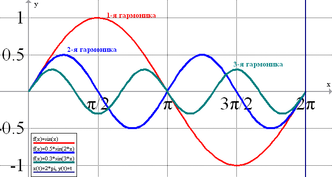
Fig. 8 Periods (frequencies) of harmonic components of the Fourier series (here T=2π)
Accordingly, the frequencies of harmonic components are multiples of 1/T. That is, frequencies of harmonic components Fk are Fk= k\T, where k runs values from 0 to ∞, for example, k=0 F0=0; k=1 F1=1\T; k=2 F2=2\T;k=3 F3=3\T;…. Fk= k\T (at zero frequency, a constant component).
Let our initial function, is a signal recorded during T=1 sec. Then the period of the first harmonic will be equal to the duration of our signal T1=T=1 sec and the frequency of the harmonic is equal to 1 Hz. The period of the second harmonic will be equal to the duration of our signal divided by 2 (T2=T/2=0.5 sec.) and the frequency is equal to 2 Hz. For the third harmonic, T3=T/3 sec and the frequency is 3 Hz. And so on.
The step between harmonics in this case is 1 Hz.
Thus, a signal with a duration of 1 sec can be decomposed into harmonic components (to obtain a spectrum) with a frequency resolution of 1 Hz.
To increase the resolution by a factor of 2 to 0.5 Hz, it is necessary to increase the duration of measurement by a factor of 2 to 2 sec. A 10-second signal can be decomposed into harmonic components (spectrum) with a frequency resolution of 0.1 Hz. There are no other ways to increase frequency resolution.
There is a way to artificially increase the signal duration by adding zeros to the array of samples. But it does not increase the real frequency resolution.
3. Discrete signals and discrete Fourier transform
With the development of digital technology the ways of measurement data (signals) storage have changed. Whereas previously a signal could be recorded on a tape recorder and stored on a tape in analog form, now signals are digitized and stored in files in computer memory as a set of numbers (counts).
The usual scheme of signal measurement and digitization looks as follows.
Measuring transducer —- Signal normalizer —- ADC —– Computer
(Fig.9 Schematic of the measuring channel)
The signal from the measuring transducer goes to the ADC for a period of time T. The signal readings (sampling) received during time T are transmitted to the computer and saved in the memory.
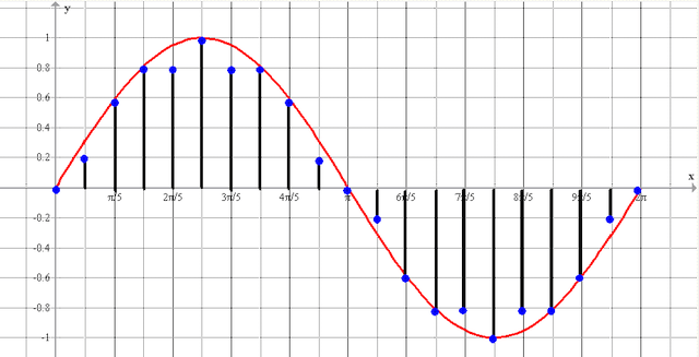
Fig.10 Digitized signal – N samples received for time T
What are the requirements to signal digitization parameters? A device which converts the input analog signal into a discrete code (digital signal) is called an analog-to-digital converter (ADC) (© Wiki).
One of the basic parameters of ADC is the maximum sampling rate – the frequency of sampling of a signal which is continuous in time. Sample rate is measured in hertz. ((© Wiki))
According to Kotelnikov’s theorem, if a continuous signal has a spectrum limited by the frequency Fmax, it can be fully and uniquely reconstructed from its discrete samples taken at time intervals T = 1/2*Fmax, ie with a frequency Fd ≥ 2*Fmax, where Fd – sampling frequency; Fmax – the maximum frequency of the signal spectrum. In other words, the frequency of signal digitization (sampling frequency of ADC) must be at least 2 times higher than the maximum frequency of the signal we want to measure.
And what will happen if we take samples with lower frequency than required by Kotelnikov’s theorem?
In this case there is an “aliasing” effect (aka stroboscopic effect, moiré effect), in which a high frequency signal after digitization turns into a low frequency signal, which in fact does not exist. In Fig. 11 the red sine wave of high frequency is the real signal. The blue sine wave of lower frequency is a fictitious signal, arising due to the fact that during the sampling time has time to pass more than half a period of the high-frequency signal.
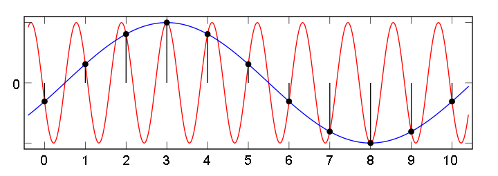
Fig. 11. Appearance of a spurious low frequency signal at an insufficiently high sampling rate
To avoid the aliasing effect, a special anti-alias filter (low-pass filter) is placed before the ADC. It passes frequencies lower than half of the ADC sampling frequency and cuts off higher frequencies.
In order to calculate signal spectrum by its discrete samples the discrete Fourier transform (DFT) is used. Note again that the spectrum of a discrete signal is “by definition” limited to a frequency Fmax smaller than half the sampling frequency Fd. Therefore, the spectrum of a discrete signal can be represented by the sum of a finite number of harmonics, in contrast to the infinite sum for the Fourier series of a continuous signal, whose spectrum can be unlimited. According to Kotelnikov’s theorem, the maximum frequency of a harmonic must be such that it accounts for at least two samples, so the number of harmonics is equal to half the number of samples of a discrete signal. That is, if there are N samples in the sample, the number of harmonics in the spectrum will be N/2.
Consider now the discrete Fourier transform (DFT).
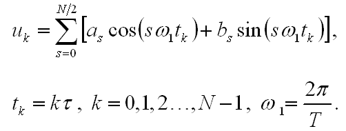
Comparing it with the Fourier series
As we can see, they coincide, except for the fact that time in the FFT is discrete and the number of harmonics is limited to N/2, which is half the number of samples.
DFT formulas are written in dimensionless integer variables k, s, where k is the number of signal samples, s is the number of spectral components.
The value s shows the number of full harmonic oscillations per period T (signal measurement duration). The discrete Fourier transform is used to find the amplitudes and phases of harmonics numerically, i.e. “on the computer”.
As it was already said above, when decomposing a non-periodic function (our signal) into Fourier series, the resulting Fourier series actually corresponds to a periodic function with period T (Fig.12).
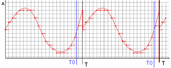
Fig.12. Periodic function f(x) with period T0, with period T>T0
As can be seen in Fig. 12, the function f(x) is periodic with period T0. However, due to the fact that the measuring sample length T is not equal to the function period T0, the function obtained as a Fourier series has a discontinuity at point T. As a result, the spectrum of this function will contain a large number of high-frequency harmonics. If the duration of measuring sample T coincided with the period of function T0, then the spectrum obtained after the Fourier transform would contain only the first harmonic (a sinusoid with a period equal to the duration of the sample), because the function f(x) is a sinusoid.
In other words, the DFT program “does not know” that our signal is a “slice of a sine wave”, but tries to represent as a series a periodic function which has a discontinuity due to the discontinuity of separate pieces of the sine wave.
As a result, harmonics appear in the spectrum, which should, in total, represent the shape of the function, including this discontinuity.
Thus, to get a “correct” spectrum of a signal which is a sum of several sinusoids with different periods, it is necessary that an integer number of periods of each sinusoid should be present on the measuring period of the signal. In practice, this condition can be met with a sufficiently long duration of signal measurement.
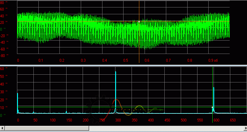
Rajah.13 Contoh fungsi isyarat ralat kinematik dan spektrum kotak gear
At shorter duration the picture will look “worse”:
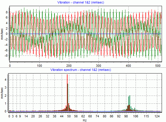
Fig.14 Example of rotor vibration function and spectrum
In practice, it can be difficult to understand where the “real components” and where the “artifacts” caused by inconsistency of component periods and signal sampling durations or “jumps and breaks” in the waveform. Of course, the words “real components” and “artifacts” are put in quotes for a reason. The presence of many harmonics on the spectrum graph does not mean that our signal actually consists of them. It is like thinking that number 7 “consists” of numbers 3 and 4. The number 7 can be thought of as the sum of 3 and 4 – that is correct.
So also our signal… or rather not even “our signal”, but a periodic function composed by repeating our signal (sample) can be represented as a sum of harmonics (sine waves) with certain amplitudes and phases. But in many cases important for practice (see figures above) it is indeed possible to relate the harmonics obtained in the spectrum also to real processes having cyclic character and contributing significantly to the form of the signal.
Some results
1. A real measured signal with T sec. duration digitized by ADC, i.e. represented by a set of discrete samples (N pieces), has a discrete non-periodic spectrum represented by a set of harmonics (N/2 pieces).
2. Isyarat diwakili oleh satu set nilai yang sah dan spektrumnya diwakili oleh satu set nilai yang sah. Frekuensi harmonik adalah positif. Hanya kerana secara matematik lebih mudah untuk mewakili spektrum dalam bentuk kompleks menggunakan frekuensi negatif tidak bermakna "ini betul" dan "ini adalah cara anda harus sentiasa melakukannya".
3. Isyarat yang diukur pada masa T hanya ditentukan pada masa T. Apa yang berlaku sebelum kita mula mengukur isyarat dan apa yang akan berlaku selepas itu tidak diketahui oleh sains. Dan dalam kes kami ia tidak menarik. FFT isyarat terhad masa memberikan spektrum "sebenar", dalam erti kata bahawa dalam keadaan tertentu ia membolehkan untuk mengira amplitud dan kekerapan komponennya.
