Understanding Harmonics in Vibration Analysis


Why integer multiples of shaft speed appear in vibration spectra — and how the pattern of 1×, 2×, 3×… harmonics reveals the precise nature of machinery faults from unbalance and misalignment to looseness and rubs.
Harmonic Frequency Calculator
Calculate harmonics and common fault frequencies for any shaft speed
Harmonic Spectrum
Visual frequency map and complete harmonic table
to see harmonic frequencies
Fault Signature Patterns — Quick Identification
Each machinery fault produces a characteristic harmonic pattern visible in the vibration spectrum
| Fault Condition | Dominant Harmonics | Amplitude Pattern | Direction | Phase Behavior | Distinguishing Feature |
|---|---|---|---|---|---|
| Mass unbalance | 1× | 1× ≫ all others | Radial | Stable; follows heavy spot | Clean single peak; proportional to speed² |
| Bent shaft | 1× + 2× | Both high | Axial + Radial | 1× phase 180° between ends (axial) | High axial 1×; not correctable by balancing |
| Angular misalignment | 1× (axial) | High axial 1× at coupling | Axial dominant | 180° across coupling (axial) | Axial 1× at coupling > radial |
| Parallel misalignment | 2× (radial) | 2× ≈ or > 1×; 3× may appear | Radial dominant | 180° across coupling (radial) | 2× ratio to 1× is diagnostic |
| Looseness — structural (Type A) | 1× | Directional — higher in loose direction | Directional | Unstable; may wander | Amplitude changes with bolt torque |
| Looseness — rotating (Type B) | 1×, 2×, 3×…n× | Rich harmonic series + ½× | Radial | Unstable; erratic | Sub-harmonics (½×, ⅓×) are key differentiator |
| Looseness — bearing seat (Type C) | Many harmonics + sub | Floor noise rise with many peaks | Radial | Very unstable | Broadband noise floor elevation |
| Soft foot | 1× + 2× | 1× changes with bolt torque | Vertical dominant | Shifts with bolt tightening | 1× amplitude changes when bolts loosened individually |
| Rotor rub (light, partial) | ½×, 1×, 2×…n× | Many high-order harmonics | Radial | Erratic; thermal drift | ½× and ⅓× sub-harmonics; thermal vector drift |
| Rotor rub (full annular) | ½×, ⅓×, ¼× dominant | Sub-harmonics > 1× | Radial | Chaotic | Sub-synchronous dominance; reverse precession |
| Oil whirl | 0.42–0.48× | Sub-synchronous peak just below ½× | Radial | Forward precession | Frequency tracks at ~0.43× RPM; speed-dependent |
| Oil whip | ≈ 1st critical | Locked at 1st critical regardless of speed | Radial | Forward precession | Frequency locks; catastrophic if unaddressed |
| Gear mesh | GMF, 2×GMF, 3×GMF | GMF = #teeth × RPM + sidebands | Radial + Axial | N/A (forced) | Sidebands at shaft speed identify damaged gear |
| Blade/vane pass | BPF, 2×BPF | BPF = #blades × RPM | Radial + Axial | N/A (forced) | Normal; high amplitude = clearance or resonance issue |
| Stator eccentricity | 2FL (100/120 Hz) | 2× line frequency dominant | Radial | N/A | Disappears instantly on power cut |
| Rotor bar defect | 1× with pole pass sidebands | Sidebands at slip freq × poles | Radial | Modulated | Zoom around 1× reveals evenly-spaced sidebands |
| VFD-induced | Switching freq harmonics | Non-synchronous peaks at PWM freq | Radial | N/A | Frequency independent of shaft speed |
| Frequency | Designation | Common Causes | Severity |
|---|---|---|---|
| 0.42–0.48× | Oil whirl | Insufficient bearing load; excessive clearance; light shaft | Critical — can lead to oil whip |
| ½× (0.50×) | Half-order | Rub, looseness (Type B/C), cracked shaft (rare), belt issues | Significant — investigate immediately |
| ⅓× (0.33×) | Third-order sub | Full annular rub; severe looseness; fluid-induced instability | Severe — dangerous condition |
| ¼× (0.25×) | Quarter-order sub | Full rub with locked orbit; extreme looseness | Very severe — shutdown may be needed |
| 1.5× (3/2×) | 3/2 order | Oil whirl combined with unbalance | Monitor closely |
| 2.5×, 3.5×… | Half-order family | Looseness with strong rub component | Combined fault mechanisms |
Definition: What is a Harmonic?
In vibration analysis, a harmonic is a frequency that is an exact integer multiple of a fundamental frequency. In rotating machinery, the fundamental frequency is typically the shaft rotational speed, referred to as the 1st harmonic or 1×. The subsequent harmonics are integer multiples: 2× (twice shaft speed), 3× (three times), and so on. These frequencies are also called orders of running speed, or synchronous harmonics because they are precisely synchronized with shaft rotation.
For example, if a motor operates at 1,800 RPM (30 Hz), its harmonics appear at 60 Hz (2×), 90 Hz (3×), 120 Hz (4×), 150 Hz (5×), and so forth. The harmonic series is theoretically infinite, but in practice, amplitude decreases at higher orders and only the first several harmonics carry diagnostic information.
Harmonics are integer multiples of shaft speed (2×, 3×, 4×…). Sub-harmonics are fractional multiples (½×, ⅓×, ¼×) and always indicate severe mechanical problems. Non-synchronous peaks are frequencies unrelated to shaft speed — such as bearing fault frequencies, gear mesh frequencies, line frequency (50/60 Hz), or natural frequencies — and require different diagnostic approaches. A peak at 3.57× RPM is NOT a harmonic; it is likely a bearing fault frequency.
Why Are Harmonics Generated?
In a perfectly linear system excited by a pure sinusoidal force (such as a perfectly balanced, perfectly aligned rotor in perfect bearings), only the 1× fundamental would appear. Real machinery is never perfectly linear. Harmonics appear whenever the vibration waveform is distorted from a pure sine wave — whenever the system response is non-linear or the forcing function itself is non-sinusoidal.
The Mathematics: Fourier's Theorem
Fourier's theorem states that any periodic waveform — no matter how complex — can be decomposed into a sum of sine waves at the fundamental frequency and its integer multiples, each with a specific amplitude and phase. The FFT (Fast Fourier Transform) algorithm used by vibration analyzers performs this decomposition computationally, revealing the harmonic content of the signal.
A pure sine wave has only a single frequency component. A square wave contains all odd harmonics (1×, 3×, 5×, 7×…) with amplitudes decreasing as 1/n. A sawtooth wave contains all harmonics with amplitudes decreasing as 1/n. The specific shape of the distortion determines which harmonics appear — this is what makes harmonic analysis so diagnostically powerful.
Physical Mechanisms That Generate Harmonics
- Waveform clipping / truncation: When shaft movement is physically constrained (bearing housing, rub contact), the resulting waveform is clipped, generating harmonics. More severe clipping produces more harmonics.
- Asymmetric stiffness: If system stiffness differs between positive and negative halves of the vibration cycle (cracked shaft opening/closing, misalignment creating different tension/compression stiffness), even harmonics (2×, 4×, 6×) are generated.
- Impact events: Periodic impacts (loose bolts, bearing defect impacts) create sharp, short-duration waveforms that are extremely rich in harmonic content — like how a drum stick produces many overtones.
- Non-linear restoring forces: When stiffness changes with displacement (bearings under varying load, progressive-rate rubber mounts), the response to a sinusoidal force contains harmonics.
- Parametric excitation: When system properties vary periodically at a frequency related to shaft speed, they can generate harmonics and sub-harmonics of the excitation frequency.
The pattern of which harmonics are present, their relative amplitudes, and which are absent tells the analyst what physical mechanism generates the non-linearity. Experienced analysts examine the complete harmonic structure of the spectrum — not just overall vibration level — to identify specific fault mechanisms.
Detailed Fault Signatures — Harmonic Patterns
1× Dominant — Unbalance
A dominant peak at 1× with minimal higher harmonics is the classic signature of mass unbalance. The unbalance force is inherently sinusoidal (it rotates with the shaft at 1× frequency), producing a clean single peak in the frequency domain.
Diagnostic Details
- Amplitude: Proportional to speed² (double speed → 4× amplitude) and proportional to unbalance mass
- Phase: Stable, repeatable, single-valued. Changes predictably with trial weight addition — this is the foundation of all balancing procedures
- Direction: Primarily radial; axial 1× is low unless rotor has significant overhang
- Confirmation: Response to trial weights confirms unbalance. If 1× doesn't respond to trial weights, consider bent shaft, eccentricity, or resonance
Several conditions produce high 1× that is NOT correctable by balancing: bent shaft, shaft eccentricity, electrical runout on proximity probes, rotor bow from thermal effects, coupling eccentricity, and resonance amplification. Always verify the diagnosis before attempting to balance.
2× Dominant — Misalignment
A strong 2nd harmonic, often comparable in amplitude to or exceeding the 1× peak, is the primary indicator of shaft misalignment. Misalignment forces the shaft through a non-sinusoidal path during each revolution, creating the distortion that generates 2× and sometimes higher harmonics.
Angular vs. Parallel Misalignment
- Angular misalignment: Shaft centerlines intersect at an angle at the coupling. Produces high 1× axial vibration. Phase across coupling shows ~180° shift in the axial direction.
- Parallel (offset) misalignment: Shaft centerlines are parallel but offset. Produces high 2× radial vibration, often with 2× ≥ 1×. Severe cases generate 3× and 4×. Radial phase across coupling shows ~180° shift.
- Combined: In practice, both usually coexist, producing a mix of the signatures.
The 2×/1× Ratio as a Diagnostic Indicator
| 2×/1× Ratio | Likely Condition | Action |
|---|---|---|
| < 0.25 | Normal; 2× present at low level in most machines | No action required |
| 0.25 – 0.50 | Mild misalignment possible; normal for some coupling types | Check alignment; compare with baseline |
| 0.50 – 1.00 | Significant misalignment probable | Perform precision laser alignment |
| > 1.00 | Severe misalignment; 2× exceeds 1× | Urgent — realign; check coupling and pipe strain |
Multiple Harmonics — Mechanical Looseness
A rich series of running speed harmonics (1×, 2×, 3×, 4×, 5×… to 10× or more) indicates mechanical looseness. The impacts, rattling, and non-linear contact/separation cycles generate extreme waveform distortion that decomposes into many harmonic components.
Three Types of Looseness
- Type A — Structural: Loose machine-to-foundation connection (soft foot, cracked base, loose anchor bolts). Produces directional 1× (higher in the loose direction). Key test: tighten/loosen individual bolts while monitoring 1× amplitude.
- Type B — Component: Loose bearing liner in cap, loose cap on housing, excessive bearing clearance. Produces a family of harmonics, often with sub-harmonics (½×). Sub-harmonics are the key differentiator from misalignment.
- Type C — Bearing seat: Loose impeller on shaft, loose coupling hub, excessive bearing clearance allowing rotor to bounce. Produces many harmonics with broadband noise floor elevation.
The presence of sub-harmonics (½×, ⅓×) is the most reliable differentiator between looseness and misalignment. Misalignment generates 2× and 3× but rarely produces sub-harmonics. Looseness (Type B and C) characteristically generates ½× because the rotor contacts one side of the bearing on one half-revolution and bounces to the other on the next — creating a pattern that repeats every two revolutions, hence ½×.
Other Harmonic-Generating Conditions
Bent Shaft
Produces both 1× and 2× vibration with high axial component. Unlike misalignment, a bent shaft shows 1× that cannot be corrected by balancing (geometric eccentricity, not mass distribution) and ~180° axial phase difference between shaft ends. The 2× comes from asymmetric stiffness as the bend opens and closes during rotation.
Reciprocating Machinery
Engines, compressors, and reciprocating machines inherently generate rich harmonic spectra because piston/crankshaft motion is fundamentally non-sinusoidal. The harmonic pattern depends on cylinder count, firing order, and stroke type (2-stroke vs. 4-stroke).
Rotor Rub
A partial rub (contact for a portion of each revolution) produces many high-order harmonics — sometimes to 10×, 20×, or more. A full annular rub (continuous 360° contact) generates dominant sub-harmonics (½×, ⅓×, ¼×) through reverse precession mechanisms.
Electrical Issues in Motors
AC motors generate vibration at multiples of line frequency (50 or 60 Hz) independently of shaft speed. The most common is 2× line frequency (100 Hz in 50 Hz systems, 120 Hz in 60 Hz systems). This is NOT a harmonic of shaft speed — it's a harmonic of line frequency, which is the key to distinguishing electrical from mechanical vibration. The power cut test is definitive: electrical vibration drops instantly when power is removed, mechanical vibration persists during coast-down.
Rotor bar defects produce sidebands around 1× spaced at the pole pass frequency (slip frequency × number of poles). These sidebands are very close to 1× (within 1–5 Hz), requiring high-resolution zoom FFT analysis to resolve.
Non-Synchronous Frequencies — Not True Harmonics
Several important frequencies are sometimes confused with harmonics but are actually independent of shaft speed:
| Frequency Type | Formula | Relationship to RPM | Notes |
|---|---|---|---|
| Bearing fault frequencies | BPFO, BPFI, BSF, FTF | Non-integer multiples (e.g. 3.57×, 5.43×) | Always non-synchronous; depend on bearing geometry |
| Gear mesh frequency | GMF = #teeth × RPM | Integer but very high order | Technically a harmonic but analyzed separately |
| Blade/vane pass | BPF = #blades × RPM | Integer multiple | Normal; excessive amplitude indicates problem |
| Line frequency | FL = 50 or 60 Hz | Not related to RPM | Electrical; disappears on power cut |
| Natural frequencies | fn = √(k/m)/2π | Fixed; not related to RPM | Constant frequency regardless of speed changes |
| Belt frequencies | fbelt = RPM×π×D/L | Sub-synchronous (< shaft speed) | Belt frequency and its harmonics 2×, 3×, 4× BF |
Analysis Guide — How to Interpret Harmonic Patterns
Step 1: Identify the Fundamental (1×)
Locate the 1× peak corresponding to shaft rotational speed. Verify using a tachometer or motor nameplate. In variable-speed machines, 1× must be identified precisely for each measurement.
Step 2: Catalog All Peaks
For each significant peak, determine: is it an exact integer multiple of 1× (true harmonic)? A fractional multiple (sub-harmonic)? Unrelated to shaft speed (non-synchronous)? Use analyzer harmonic cursor features for efficiency.
Step 3: Examine the Amplitude Pattern
- Which harmonic is dominant? → Points to specific fault
- How many harmonics are present? → More = more severe distortion
- Does 2× exceed 1×? → Likely misalignment
- Are sub-harmonics present? → Looseness, rub, or oil whirl
- Is amplitude decreasing with order (1/n decay)? → Typical for looseness
Step 4: Check Directionality
- High radial, low axial: Unbalance or looseness
- High axial: Misalignment (especially angular) or bent shaft
- Directional radial: Structural looseness (higher in loose direction)
Step 5: Trend Over Time
- Are harmonic amplitudes increasing? → Fault is progressing
- Are new harmonics appearing? → New fault mechanism developing
- Is the noise floor rising? → General wear or late-stage failure
Step 6: Correlate with Phase Data
- Unbalance: 1× phase is stable and repeatable
- Misalignment: 1× or 2× phase shows ~180° across coupling
- Looseness: Phase is unstable, may shift randomly between measurements
Case Studies — Real-World Harmonic Analysis
Machine: 30 kW motor driving centrifugal pump at 2960 RPM via flexible coupling. Overall vibration: 6.2 mm/s at motor drive-end bearing.
Spectrum: 1× = 4.1 mm/s, 2× = 3.8 mm/s, 3× = 1.2 mm/s. The 2×/1× ratio = 0.93.
Direction: High radial 2× at both drive-end bearings. Axial 1× at coupling: motor = 2.8 mm/s, pump = 3.1 mm/s with 165° phase difference.
Diagnosis: Combined angular and parallel misalignment. The 2×/1× ratio approaching 1.0, high axial readings, and ~180° phase across coupling all confirm. NOT unbalance — even though 1× is elevated, the 2× pattern is the real story.
Action: Laser alignment performed. Post-alignment: 1× = 0.8 mm/s, 2× = 0.3 mm/s. Overall dropped to 1.1 mm/s — an 82% reduction.
Machine: Centrifugal fan at 1480 RPM. Vibration: 8.5 mm/s. Previous balancing attempt reduced 1× but overall vibration remained high.
Spectrum: 1× = 2.1 mm/s (low after balancing), ½× = 1.8 mm/s, 2× = 3.2 mm/s, 3× = 2.5 mm/s, 4× = 1.8 mm/s, 5× = 1.1 mm/s, 6× = 0.7 mm/s.
Diagnosis: Mechanical looseness (Type B). The harmonic family with ½× sub-harmonic is the signature. Balancing corrected 1× but couldn't address the looseness-generated harmonics that dominate overall vibration.
Action: Inspection revealed bearing housing 0.08 mm loose in pedestal bore. Housing rebored and new bearing fitted. Post-repair: all harmonics dropped to baseline. Overall: 1.4 mm/s.
Machine: 4-pole, 50 Hz induction motor at 1485 RPM driving a screw compressor. Vibration increased from 2.0 to 5.5 mm/s over 3 months.
Spectrum: Dominant peak at 100 Hz (= 2FL). Also: 1× at 24.75 Hz = 1.2 mm/s, sidebands around 1× at ±1.0 Hz spacing.
Key Test: Power cut — the 100 Hz peak dropped to zero within one revolution. The 1× sidebands persisted during coast-down.
Diagnosis: Two problems: (1) Electrical — stator eccentricity causing 2FL. (2) Mechanical — 1× sidebands at ±1.0 Hz (= pole pass frequency for 4-pole motor with 1.0% slip) suggest developing rotor bar defect.
Action: Motor sent for rewind. Confirmed: 2 broken rotor bars + stator eccentricity from base sag. After rewind and shimming: vibration 1.6 mm/s.
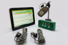
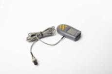
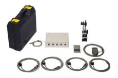
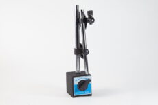
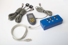
The Balanset-1A and Balanset-4 provide real-time FFT spectrum analysis with harmonic cursor tracking, enabling field identification of 1×, 2×, 3× patterns and fault diagnosis. The devices combine vibration analysis for diagnostics and precision balancing for correction — identifying the problem and fixing it with one instrument.
Professional Vibration Analysis & Balancing
Diagnose harmonic patterns and balance rotors in the field with Vibromera's portable devices — FFT spectrum, phase measurement, and ISO-compliant balancing in one instrument.
Browse Equipment →