7.3 Balancing procedure
Balancing is performed for mechanisms in good technical condition and correctly mounted. Otherwise, before the balancing the mechanism must be repaired, installed in proper bearings and fixed. Rotor should be cleaned of contaminants that can hinder from balancing procedure.
Before balancing measure vibration in Vibration meter mode (F5 button) to be sure that mainly vibration is 1x vibration.
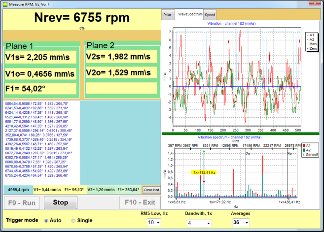
Fig. 7.10. Vibration meter mode. Checking overall (V1s,V2s) and 1x (V1o,V2o) vibration.
If the value of the overall vibration V1s (V2s) is approximately equal to the magnitude of the
vibration at rotational frequency (1x vibration) V1o (V2o), it can be assumed that the main contribution to the vibration mechanism pays an imbalance of the rotor. If the value of the overall vibration V1s (V2s) is much higher than the 1x vibration component V1o (V2o), it is recommended to check the condition of a mechanism – condition of bearings, its mount on the base, the lack of grazing for the fixed parts of the rotor during rotation, etc.
You should also pay attention to the stability of the measured values in Vibration meter mode – the amplitude and phase of the vibration should not vary by more than 10-15% in the measurement process. Otherwise, it can be assumed that the mechanism is running close-to-resonance domain. In this case, change the speed of rotation of the rotor, and if this is not possible – change the conditions of installation of the machine on the foundation (for example, temporarily setting on spring supports).
For rotor balancing influence coefficient method of balancing (3-run method) should be taken.
Trial runs are done to determine the effect of trial mass on vibration change, mass and place (angle) of installation of correction weights.
First determine the original vibration of a mechanism (first start without weight), and then set the trial weight to the first plane and made the second start. Then, remove the trial weight from the first plane, set in a second plane and made the second start.
The program then calculates and indicates on the screen the weight and location (angle) of installation of correction weights.
When balancing in a single plane (static), the second start is not required.
Trial weight is set to an arbitrary location on the rotor where it is convenient, and then the actual radius is entered in the setup program.
(Position Radius is used only for calculating the unbalance amount in grams * mm)
Important!
Mass of the trial weight is selected so that after its installation phase (> 20-30°) and (20-30%) the amplitude of vibration change significantly. If changes are too small, the error increases greatly in subsequent calculations. Conveniently set trial mass at the same place (the same angle) as the phase mark.
Important!
After each test run trial mass are removed! Correction weights set at an angle calculated from the place of trial weight installation in the direction of rotation of the rotor!
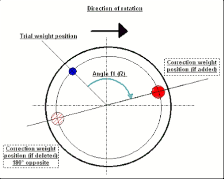
Fig. 7.11. Correction weight mounting.
Recommended!
Before performing dynamic balancing, it is recommended to make sure that static imbalance is not too high. For rotors with horizontal axis, the rotor can be manually rotated by an angle of 90 degrees from the current position. If the rotor is statically unbalanced, it will be rotated to a position of equilibrium. Once the rotor will assume the position of equilibrium, it is necessary to set the weight balancing in the top point approximately in the middle part of the rotor length. Weight of the weight should be chosen in such a way that the rotor is not moving in any position.
Such pre-balancing will reduce the amount of vibration at the first start of strongly unbalanced rotor.
Sensor installation and mounting.
Vibration sensor must be installed on the machine in the selected measuring point and connected to the input X1 of the USB interface unit.
There are two mounting configurations
• Magnets
• Threaded studs M4
Optical tacho sensor should be connected to the input X3 of the USB interface unit. Furthermore, for use of this sensor a special reflecting mark should be applied on surface of a rotor.
Detailed requirements on site selection of the sensors and their attachment to the object when balancing are set out in Annex 1.
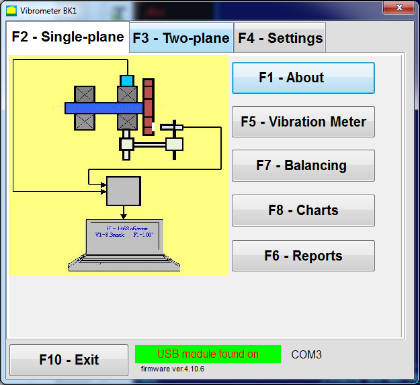
Fig. 7.12. “Single plane balancing“
To start working on the program in the “Single-Plane balancing” mode, click on the “F2-Single-plane” button (or press the F2 key on the computer keyboard).
.
Then click on the “F7 – Balancing” button, after which the Single Plane balancing archive window will appear, in which the balancing data will be saved (see Fig. 7.13).

Fig. 7.13 The window for selecting the balancing archive in single plane.
In this window, you need to enter data on the name of the rotor (Rotor name), place of rotor installation (Place), tolerances for vibration and residual imbalance (Tolerance), date of measurement. This data is stored in a database. Also, a folder Arc### is created in, where ### is the number of the archive in which the charts, a report file, etc. will be saved. After the balancing is completed, a report file will be generated that can be edited and printed in the built-in editor.
After entering the necessary data, you need to click the “F10-OK” button, after which the “Single-Plane balancing” window will open (see Fig. 7.13)

Fig. 7.14. Single plane. Balancing settings
In the left side of this window displays the data of vibration measurements and the measurement control buttons “Run # 0”, “Run # 1”, “RunTrim”.
In the right side of this window there are three tabs
The “Balancing settings” tab is used to enter the balancing settings:
1. “Influence coefficient” –
• “New Rotor” – selection of the balancing of the new rotor, for which there are no stored balancing coefficients and two runs are required to determine the mass and installation angle of the correction weight.
• “Saved coeff.” – selection of the rotor re-balancing, for which there are saved balancing coefficients and only one run is required for determining the weight and installation angle of the corrective weight.
2. “Trial weight mass” –
• “Percent” – corrective weight is calculated as a percentage of the trial weight.
• “Gram” – the known mass of the trial weight is entered and the mass of the corrective weight is calculated in grams or in oz for Imperial system.
Attention!
If it is necessary to use the “Saved coeff.” Mode for further work during initial balancing, the trial weight mass must be entered in grams or oz, not in %. Scales are included in the delivery package.
3. “Weight Attachment Method”
• “Free position” – weights can be installed in an arbitrary angular positions on the circumference of the rotor.
• “Fixed position” – weight can be installed in fixed angular positions on the rotor, for example, on blades or holes (for example 12 holes – 30 degrees), etc. The number of fixed positions must be entered in the appropriate field. After balancing, the program will automatically split the weight into two parts and indicate the number of positions on which it is necessary to establish the masses obtained.

Fig. 7.15. Result tab. Fixed position of correction weight mounting.
Z1 and Z2 – positions of corrective weights installed, calculated from Z1 position according rotation direction. Z1 is position of trial weight was installed.
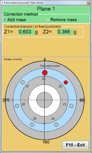
Fig. 7.16 Fixed positions. Polar diagram.
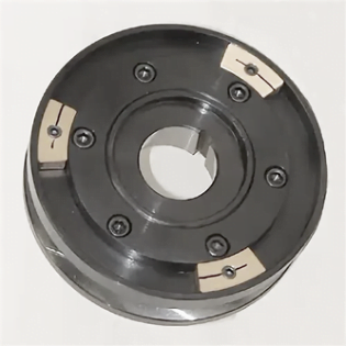
Fig. 7.17 Grinding wheel balancing with 3 counterweights
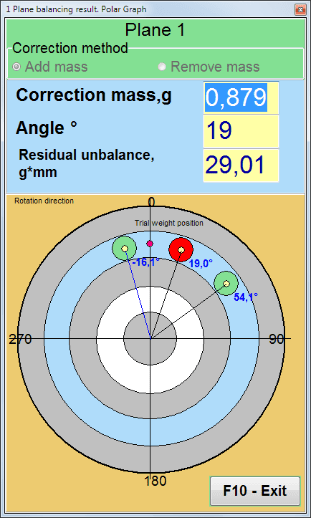
Fig. 7.18 Grinding wheel balancing. Polar graph.
Balancing with additional start to eliminate the influence of the eccentricity of the mandrel (balancing arbor). Mount the rotor alternately at 0° and 180° relative to the. Measure the unbalances in both positions.
• Balancing tolerance
Entering or calculating residual imbalance tolerances in g x mm (G-classes)
• Use Polar Graph
Use polar graph to display balancing results
As noted above, “New Rotor” balancing requires two test run and at least one trim run of the balancing machine.
After installing the sensors on the balancing rotor and entering the settings parameters, it is necessary to turn on the rotor rotation and, when it reaches working speed, press the “Run#0” button to start measurements.
The “Charts” tab will open in the right panel, where the wave form and spectrum of the vibration will be shown (Fig. 7.18.). In the bottom part of the tab, a history file is kept, in which the results of all starts with a time reference are saved. On disk, this file is saved in the archive folder by the name memo.txt
Attention!
Before starting the measurement, it is necessary to turn on the rotation of the rotor of the balancing machine (Run#0) and make sure that the rotor speed is stable.
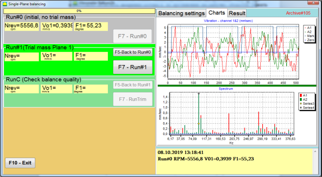
Fig. 7.19. Balancing in one plane. Initial run (Run#0). Charts Tab
After measurement process finished, in the Run#0 section in the left panel the results of measuring appears – the rotor speed (RPM), RMS (Vo1) and phase (F1) of 1x vibration.
The “F5-Back to Run#0” button (or the F5 function key) is used to return to the Run#0 section and, if necessary, to repeat measure the vibration parameters.
Before starting the measurement of vibration parameters in the section “Run#1 (Trial mass Plane 1), a trial weight should be installed according “Trial weight mass” field. (see Fig. 7.10).
The goal of installing a trial weight is to evaluate how the vibration of the rotor changes when a known weight is installed at a known place (angle). Trial weight must changes the vibration amplitude by either 30% lower or higher of initial amplitude or change phase by 30 degrees or more of initial phase.
2. If it is necessary to use the “Saved coeff.” balancing for further work, the place (angle) of installation of the trial weight must be the same as the place (angle) of the reflective mark.
Turn on the rotation of the rotor of the balancing machine again and make sure that it rotation frequency is stable. Then click on the “F7-Run#1” button (or press the F7 key on the computer keyboard). “Run#1 (Trial mass Plane 1)” section (see Fig. 7.18)
After the measurement in the corresponding windows of the “Run#1 (Trial mass Plane 1)” section, the results of measuring the rotor speed (RPM), as well as the value of the RMS component (Vо1) and phase (F1) of 1x vibration appearing.
At the same time, the “Result” tab opens on the right side of the window (see Fig. 7.13).
This tab displays the results of calculating the mass and angle of corrective weight, which must be installed on the rotor to compensate imbalance.
Moreover, in the case of using the polar coordinate system, the display shows the value of the mass (M1) and the installation angle (f1) of the correction weight.
In the case of “Fixed positions” the numbers of the positions (Zi, Zj) and trial weight splitted mass will be shown.
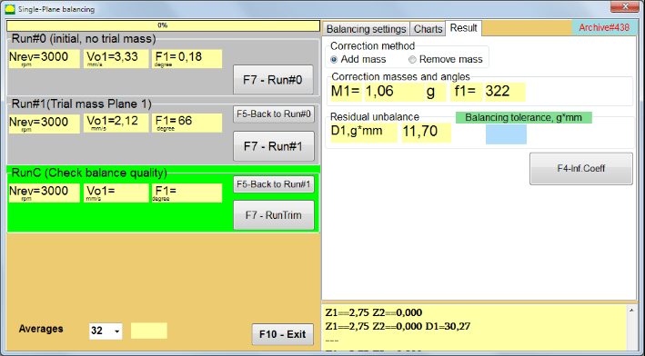
Fig. 7.20. Balancing in one plane. Run#1 and balancing result.
If Polar graph is checked polar diagram will be shown.
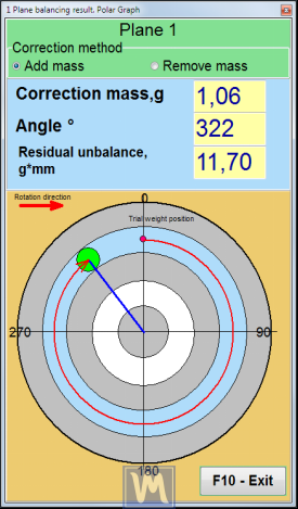
Fig. 7.21. The result of balancing. Polar graph.
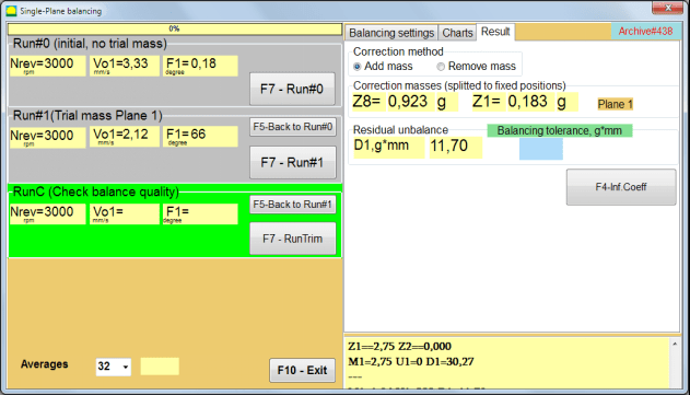
Fig. 7.22. The result of balancing. Weight splitted (fixed positions)
Also if “Polar graph” was checked, Polar graph will be shown.
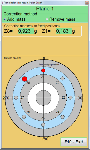
Fig. 7.23. Weight splitted on fixed positions. Polar graph
Attention!:
1. After completing the measurement process at the second run (“Run#1 (Trial mass Plane 1)”) of the balancing machine, it is necessary to stop the rotation and remove installed trial weight. Then install (or remove) the corrective weight on the rotor according result tab data.
If the trial weight was not removed, you need to switch to the “Balancing settings” tab and turn on the checkbox in “Leave trial weight in Plane1”. Then switch back to the “Result” tab. The weight and installation angle of the correction weight are recalculated automatically.
2. The angular position of the corrective weight is performed from the place of installation of the trial weight. The direction of reference of the angle coincides with the direction of rotation of the rotor.
3. In the case of “Fixed position” – the 1st position (Z1), coincides with the place of installation of the trial weight. The counting direction of the position number is in the direction of rotation of the rotor.
4. By default the corrective weight will be added to the rotor. This is indicated by the label set in the “Add” field. If removing the weight (for example, by drilling), you must set a mark in the “Delete” field, after which the angular position of the correction weight will automatically change by 180º.
After installing the correction weight on the balancing rotor in the operating window (see Fig. 7.15), it is necessary to carry out a RunC (trim) and evaluate the effectiveness of the performed balancing.
Attention!
Before starting the measurement on the RunC, it is necessary to turn on the rotation of the rotor of the machine and make sure that it has entered the operating mode (stable rotation frequency).
To perform vibration measurement in the “RunC (Check balance quality)” section (see Fig. 7.15), click on the “F7 – RunTrim” button (or press the F7 key on the keyboard).
Upon successful completion of the measurement process, in the “RunC (Check balance quality)” section in the left panel, the results of measuring the rotor speed (RPM) appear, as well as the value of the RMS component (Vo1) and phase (F1) of 1x vibration.
In the “Result” tab, the results of calculating the mass and installation angle of the additional corrective weight are displayed.
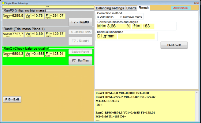
Fig. 7.24. Balancing in one plane. Performing a RunTrim. Result Tab
This weight can be added to the correction weight that is already mounted on the rotor to compensate for the residual imbalance. In addition, the residual rotor unbalance achieved after balancing is displayed in the lower part of this window.
In the case when the amount of residual vibration and / or residual unbalance of the balanced rotor meets the tolerance requirements established in the technical documentation, the balancing process can be completed.
Otherwise, the balancing process may continue. This allows the method of successive approximations to correct possible errors that may occur during the installation (removal) of the corrective weight on a balanced rotor.
When continuing the balancing process on the balancing rotor, it is necessary to install (remove) additional corrective mass, the parameters of which are indicated in the section “Correction masses and angles”.
The “F4-Inf.Coeff” button in the “Result” tab (Fig. 7.23,) is used to view and store in the computer memory the coefficients of rotor balancing (Influence coefficients) calculated from the results of calibration runs.
When it is pressed, the “Influence coefficients (single plane)” window appears on the computer display (see Fig. 7.17), in which balancing coefficients calculated from the results of calibration (test) runs are displayed. If during the subsequent balancing of this machine it is supposed to use the “Saved coeff.” Mode, these coefficients must be stored in the computer memory.
To do this, click the “F9 – Save” button and go to the second page of the “Influence coeff. archive. Single plane.”(See Fig. 7.24)

Fig. 7.25. Balancing coefficients in the 1st plane
Then you need to enter the name of this machine in the “Rotor” column and click “F2-Save” button to save the specified data on the computer.
Then you can return to the previous window by pressing the “F10-Exit” button (or the F10 function key on the computer keyboard).
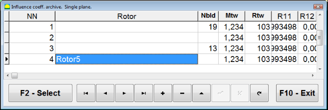
Fig. 7.26. “Influence coeff. archive. Single plane. “
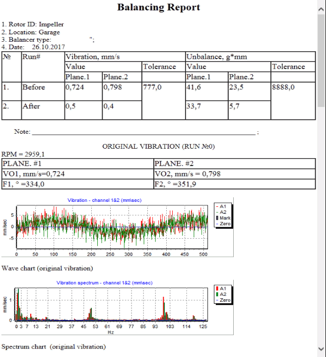
Fig. 7.26. Balancing report.
Saved coeff. balancing can be performed on a machine for which balancing coefficients have already been determined and entered into the computer memory.
Attention!
When balancing with saved coefficients, the vibration sensor and the phase angle sensor must be installed in the same way as during the initial balancing.
Input of the initial data for Saved coeff. balancing (as in the case of primary(“New rotor”) balancing) begins in the “Single plane balancing. Balancing settings.”(See Fig. 7.27).
In this case, in the “Influence coefficients” section, select the “Saved coeff” item. In this case, the second page of the “Influence coeff. archive. Single plane.”(See Fig. 7.27), which stores an archive of the saved balancing coefficients.
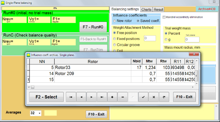
Fig. 7.28. Balancing with saved influence coefficients in 1 plane
Moving through the table of this archive using the “►” or “◄” control buttons, you can select the desired record with balancing coefficients of the machine of interest to us. Then, to use this data in current measurements, press the “F2 – Select” button.
After that, the contents of all other windows of the “Single plane balancing. Balancing settings.” are filled in automatically.
After completing the input of the initial data, you can begin to measure.
Balancing with saved influence coefficients requires only one initial run and at least one test run of the balancing machine.
Attention!
Before starting the measurement, it is necessary to turn on the rotation of the rotor and make sure that rotating frequency is stable.
To carry out the measurement of vibration parameters in the “Run#0 (Initial, no trial mass)” section, press “F7 – Run#0” (or press the F7 key on the computer keyboard).
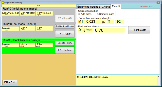
Fig. 7.29. Balancing with saved influence coefficients in one plane. Results after one run.
In the corresponding fields of “Run#0” section, the results of measuring the rotor speed (RPM), the value of the RMS component (Vо1) and phase (F1) of 1x vibration appear.
At the same time, the “Result” tab displays the results of calculating the mass and angle of the corrective weight, which must be installed on the rotor to compensate imbalance.
Moreover, in the case of using a polar coordinate system, the display shows the values of the mass and the installation angle of the correction weight.
In the case of splitting of the corrective weight on the fixed positions, the numbers of the positions of the balancing rotor and the mass of weight that need to be installed on them are displayed.
Further, the balancing process is carried out in accordance with the recommendations set out in section 7.4.2. for primary balancing.
To carry out index balancing, a special option is provided in the Balanset-1A program. When checked Mandrel eccentricity elimination an additional RunEcc section appears in the balancing window.

Fig. 7.30. The working window for Index balancing.
After running Run # 1 (Trial mass Plane 1), a window will appear
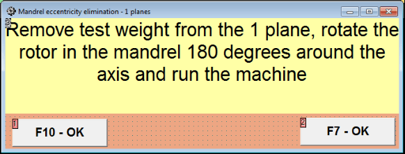
Fig. 7.31 Index balancing attention window.
After installing the rotor with an 180 turn, Run Ecc must be completed. The program will automatically calculate the true rotor imbalance without affecting the mandrel eccentricity.