Vārpstas orbītas diagrammas izpratne vibrācijas analīzē
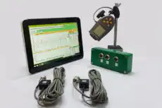


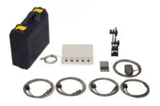



A vārpstas orbīta ir grafiks, kas attēlo trajektoriju, ko vienā vai vairākos apgriezienos iezīmē rotējošas vārpstas ģeometriskais centrs. Tas ir divdimensionāls attēlojums vārpstas kustībai tās gultņa klīrenss, it kā jūs skatītos tieši uz vārpstas galu. Šo spēcīgo diagnostikas rīku iegūst, uzstādot pāri bezkontakta tuvuma zondes 90 grādu leņķī — parasti X-Y konfigurācijā — un attēlojot to vienlaicīgos pārvietojuma signālus attiecībā viens pret otru, nevis pret laiku.
1. Kāpēc orbītas diagramma ir tik noderīga
Standarta laika viļņa forma vai FFT spektrs rāda tādu lielumu kā vibrācija vienā virzienā. Orbītas diagramma apvieno divus perpendikulārus virzienus, sniedzot pilnīgu priekšstatu par vārpstas dinamisko kustību, ļaujot analītiķiem vizualizēt kustības faktisko formu un virzienu, nevis to tikai secināt. Šis papildu dimensijas elements sniedz nenovērtējamas norādes dažādu defektu diagnosticēšanai, tāpēc orbīta ir rotora dinamika analīze — jo īpaši attiecībā uz ātrgaitas, kritiskām iekārtām, kas aprīkotas ar šķidruma plēvi slīdgultņi, piemēram, turbīnas, kompresori un lieljaudas ģeneratori.
Tā kā devēji mēra nobīdi tieši pret gultni, orbīta parāda ne tikai to, cik tālu vārpsta pārvietojas, bet arī to, kur tā atrodas savā klīrensa diapazonā — informācija, ko uz korpusa uzstādītais akselerometrs vienkārši nevar nodrošināt. Pievienojot tādu ierīci kā tahometrs vai Keyphasor marķējums iezīmē katru apgriezienu orbītā, fiksējot tā fāze un padarot precesijas virzienu nepārprotamu.
2. Kā interpretēt orbītu formas
Orbītas forma, izmērs un orientācija ir tiešie rādītāji spēkiem, kas iedarbojas uz rotoru. Prasmīgs analītiķis var diagnosticēt mašīnas stāvokli, vienkārši aplūkojot orbītas formu.
Apļveida vai elipsveida orbīta
Vienkārša apļveida vai eliptiska orbīta, kuras centrs atrodas gultnī, parasti liecina par stabilu rotora darbību, kurā dominē viena frekvence — visbiežāk nelīdzsvarotība. Orbīta būs apļveida, ja gultņu balsta stingrība abos virzienos ir vienāda (izotropiska), un eliptiska, ja stingrība horizontālā un vertikālā virzienā atšķiras (anizotropiska), kas praksē ir ļoti izplatīts gadījums, jo lielākā daļa mašīnu vertikālā virzienā ir stingrāka nekā horizontālā.
Izkropļota, 8. attēla vai banāna formas orbīta
Ja orbīta atšķiras no vienkāršas elipses, vārpstas kustību ietekmē vairāki frekvences faktori:
- A "Banāna" vai pusmēness formas orbīta bieži vien ir saistīts ar vārpstu nesakritība, kurā ir gan 1×, gan 2× frekvences.
- A astoņnieka formas ir klasiskas pazīmes, kas liecina par izteiktu 2× komponenti, – tipisks vārpstu nesakritības rādītājs. 8-veida līnija ar iekšējo cilpu bieži norāda uz nopietnāku stāvokli vai berzes klātbūtni.
Orbītas ar līkumiem vai asiem stūriem
Asas virziena izmaiņas, plakani plankumi vai "locījumi" orbītā ir spēcīgi pierādījumi par rotora un statora berze. Tie liecina, ka vārpstas kustība uz brīdi tiek ierobežota, kad tā saskaras ar nekustīgu detaļu, piemēram, gultni, blīve, vai iekārtas korpuss.
Ļoti neregulāras orbītas
Orbīta, kas ir nepastāvīga, nestabila vai šķiet pārpildīta ar „trokšņiem“, var liecināt par tādām problēmām kā nopietns mehānisks vaļīgums, šķidruma izraisīta nestabilitāte, piemēram, eļļas virpulis vai oil whip, vai arī turbulentu plūsmu apstākļi sūkņā vai kompresorā.
3. Precesijas virziens: uz priekšu vai atpakaļ
Virziens, kādā tiek izsekota orbīta, attiecībā pret vārpstas rotācijas virzienu, pats par sevi ir galvenais diagnostiskais faktors:
- Priekšējā precesija: Orbītas līnijas virzās tajā pašā virzienā kā vārpstas rotācija. Tas ir normāls rādītājs tādiem spēkiem kā nelīdzsvarotība.
- Apgriezta precesija: Orbītas trajektorija ir pretēja vārpstas rotācijas virzienam. Tas ir neparasts stāvoklis un var liecināt par vārpstas plaisa, spēcīga berze vai noteikti šķidruma izraisītas nestabilitātes veidi.
Lai atšķirtu šos divus, ir nepieciešams fāzes marķējums, kas atrodas vienu reizi apgriezienā; bez tā orbīta parāda formu, bet ne virzienu, kurā tā tiek izieta, un tādējādi zūd diagnostiskā atšķirība.
4. Orbīta lauka diagnostikā
Pastāvīgi uzstādīti tuvinājuma devēji, kas sniedz datus uzraudzības sistēmai, ir klasisks risinājums, lai noteiktu rotācijas trajektoriju lielām kritiskām iekārtām, taču pamatprincips — divi perpendikulāri pārvietojuma signāli, kas attēloti viens pret otru ar fāzes atsauci — ir vienlīdz pieejams arī lauka inženierim. Pārnēsājams divkanālu mērinstruments, piemēram, Balanset-1A vienlaikus mēra sinhrono amplitūdu un fāzi divās plaknēs, tāpēc, tiklīdz orbīta vai spektrs to ir apstiprinājis, nelīdzsvarotība ir dominējošais spēks, un šī pati struktūra tiek saglabāta arī lauka balansēšana un izlabotā stāvokļa pārbaude. Ja orbīta liecina par nevienmērīgu līdzsvarošanu, berzi vai nestabilitāti, šis secinājums liek darbu virzīt uz līdzsvarošanu vai mehānisku labojumu, nevis uz balansēšanu.
Displacement Orbit versus Velocity Orbit
The two are not the same measurement, and the difference decides what you are entitled to conclude from the picture. A pair of proximity probes reads shaft pārvietojums relative to the bearing, so the plot is a true map of where the journal sits inside its clearance, and the DC part of the same signal yields the vārpstas centra līnija. A portable two-channel analyser with accelerometers clamped to the bearing housings plots two ātrums channels against each other, in mm/s: what you see is the motion of the housing, not the position of the shaft.
What survives the change of transducer is the geometry. Shape, orientation and precession direction are set by the pattern of forces acting on the rotor rather than by the sensor, so the familiar families still appear — a smooth ellipse when 1× dominates, a crescent or figure-8 when a strong 2× component is present, flattened sides and kinks when something rubs. What does not survive is absolute position: a velocity orbit cannot tell you how much clearance is left, and it cannot be rescaled into micrometres of shaft motion. Use it in the field to identify the fault family; reach for proximity probes when the question is where the shaft is actually running.
Where the Orbit Lives in the Balanset Software
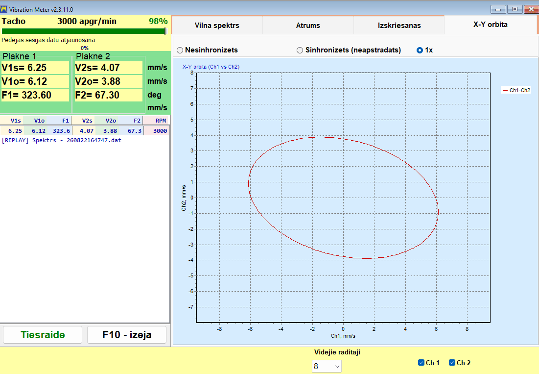
On a Balanset-1A the orbit is one tab of the vibration-meter window, opened with the F5 key from the main window; the window requires device firmware 5.5.0 or newer. The “X-Y Orbit” tab plots channel 1 on one axis against channel 2 on the other at a 1:1 axis scale, so a circle on screen is genuinely a circle and not an artefact of unequal axes. On the four-channel Balanset-4A a second orbit, for channels 3 and 4, is drawn beneath the first.
A switch above the chart decides what is drawn:
| Režīms | What is plotted | When it is the right view |
|---|---|---|
| Unsynced | The raw trajectory, with no revolution reference | No tachometer is available, or you want to see everything the signal contains |
| Sync (raw) | The most recent revolutions overlaid, aligned to the tachometer mark | Judging repeatability — a stable, closed figure means the motion repeats turn after turn |
| 1× | The rotational component alone: a clean ellipse that matches the V·o and F readings | Confirming the unbalance vector before balancing |
Without a tachometer mark the two synchronised modes have nothing to synchronise to, the program says so in the chart title, and “Unsynced” becomes the only honest view. This is the practical form of the point made in section 3: no once-per-revolution reference, no precession direction.
Reading the Numbers Beside the Orbit
The tiles next to the chart carry three values per measuring plane, and together they are the fastest sanity check available before you start interpreting shapes:
- V·s — broadband RMS velocity across the working band, in mm/s.
- V·o — the 1× component alone, at rotational frequency, in mm/s.
- F — tas fāze of that 1× component, in degrees.
The rotational component is part of the total by construction, so V·o can never exceed V·s, and the ratio between them predicts the orbit before you look at it. When V·o sits close to V·s, nearly all the energy is at 1×, the orbit collapses to a clean ellipse, and nelīdzsvarotība is the dominant force. When V·o is markedly smaller, the difference is harmonics and broadband noise — and it is exactly that residue which bends the ellipse into the crescents, figure-8s and kinks described in section 2. A badly distorted orbit reported alongside V·o ≈ V·s is a contradiction, and the instrumentation is the first thing to check.
Beneath each plane sits a stability bar: grey while the reading is still drifting, green once the coefficient of variation over the last twelve stream values falls below 10 %, orange when the spread exceeds 20 %. An orbit captured while that bar is orange is not a diagnosis — it is a photograph of a machine that has not settled.
Confirming the Shape Against the Spectrum
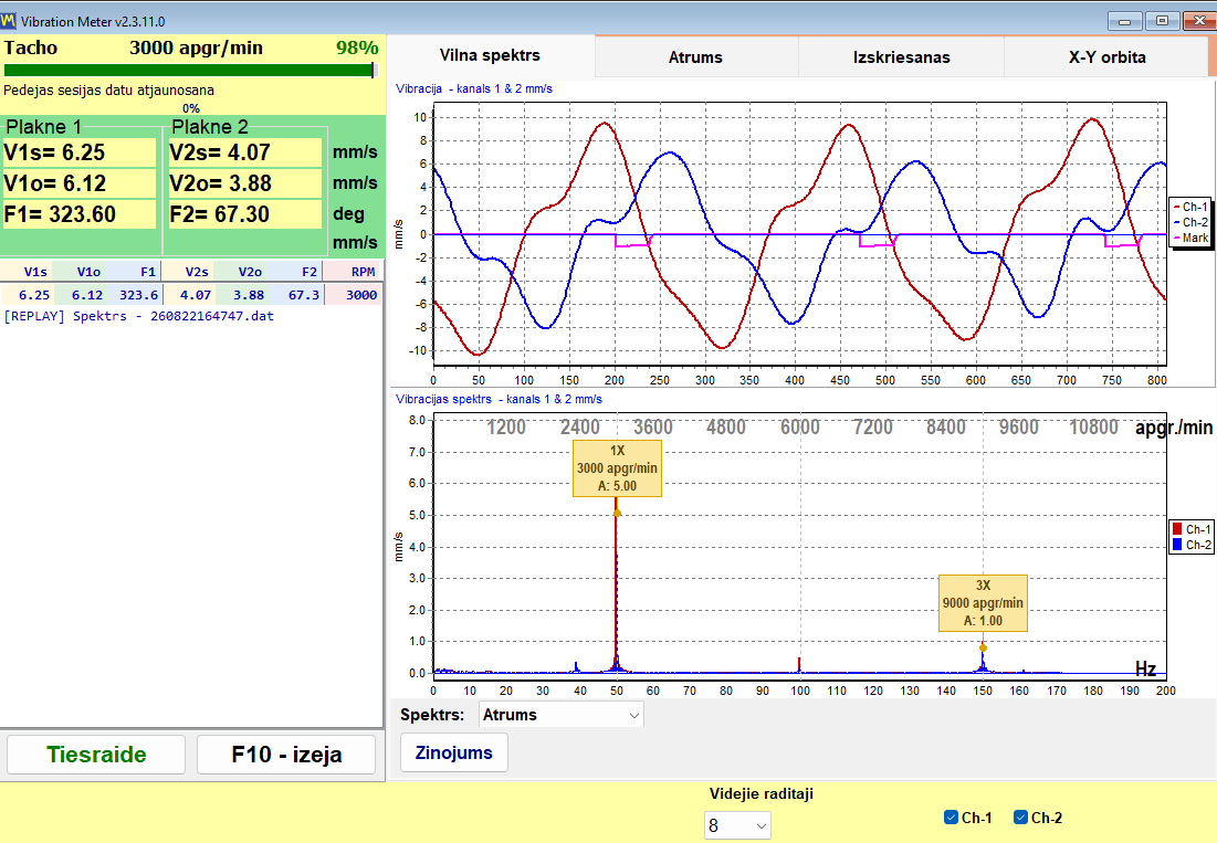
The orbit tells you that something is distorting the ellipse; the spectrum tells you which order is responsible. The “Wave Spectrum” tab of the same window shows the waveform above and the velocity spectrum below, with dashed guides placed at exact multiples of the measured rotational speed rather than at the nearest tall bar — so a peak that misses its marker is not a harmonic of shaft speed at all and belongs to bearings, gear mesh or blade pass instead. A dominant 2× beside a crescent or figure-8 orbit points at vārpstu nesakritība; a peak between 0.43× and 0.48× under a drifting, unstable orbit is the signature of eļļas virpulis; broadband content with flattened orbit sides points at a berzēt.
The selector below the chart switches the spectrum between velocity and acceleration. Velocity is the axis to use when reasoning about the orbit, because the orbit itself is drawn from the velocity channels.
Watching the Orbit Through a Resonance
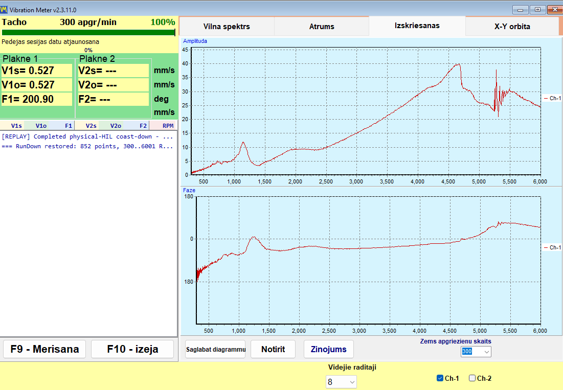
An orbit is a snapshot at one speed, and the shape can change completely a few hundred RPM away. The “Run-down” tab records the whole coast-down instead: 1× amplitude and phase are logged against falling speed, one raw value per revolution with no smoothing, down to a stop threshold that can be set anywhere between 100 and 2000 RPM and defaults to 300. A resonance announces itself as an amplitude peak accompanied by a phase rotation of roughly 180° — the same critical speed that a Kempbela diagramma predicts where an excitation line crosses a natural-frequency curve. The full run-down report keeps the X-Y orbit captured at working speed alongside those curves, so the shape and the resonance map end up in one document.
5. Ko parāda orbītas grafiks
Kopumā vienā orbītas diagrammā uzreiz var iegūt plašu informāciju:
- Vārpstas vibrācijas kopējā amplitūda.
- – Vārpstas kustības forma, kas palīdz noteikt defekta veidu.
- Precesijas virziens — uz priekšu vai atpakaļ.
- Vārpstas vidējā atrašanās vieta gultņa spēles robežās — tās vārpstas centra līnija.
Analizējot kopā ar FFT spektru un laika signāla formu, orbīta ļauj analītiķim iegūt ļoti ticamus un detalizētus diagnoze par mašīnas dinamisko uzvedību — apvienojot „cik daudz“, „kāda forma“ un „kādā virzienā“ vienā izšķirošā kopainā.