Understanding the Shaft Orbit Plot in Vibration Analysis
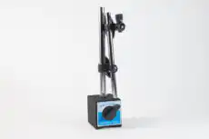

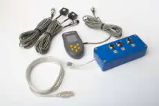
A shaft orbit is a plot that shows the path traced by a rotating shaft’s geometric centre during one or more revolutions. It is a two-dimensional view of the shaft’s motion within its bearing clearance, as if you were looking straight down the end of the shaft. This powerful diagnostic is created by mounting a pair of non-contact proximity probes 90 degrees apart — typically in an X-Y configuration — and plotting their simultaneous displacement signals against each other rather than against time.
1. Why the Orbit Plot Is So Useful
A standard time waveform or FFT spectrum shows vibration in a single direction. The orbit plot combines two perpendicular directions to give a complete picture of the shaft’s dynamic motion, letting analysts visualise the actual shape and direction of the movement rather than inferring it. That extra dimension provides invaluable clues for diagnosing a wide range of faults, which is why the orbit is a cornerstone of rotor-dynamic analysis — especially for high-speed, critical machinery fitted with fluid-film journal bearings, such as turbines, compressors, and large generators.
Because the probes measure displacement directly against the bearing, the orbit also reveals where the shaft sits within its clearance, not just how far it moves — information a casing-mounted accelerometer simply cannot provide. Adding a tachometer or Keyphasor mark stamps each revolution onto the orbit, fixing its phase and making precession direction unambiguous.
2. How to Interpret Orbit Shapes
The shape, size, and orientation of the orbit are direct indicators of the forces acting on the rotor. A skilled analyst can often diagnose a machine’s condition simply by looking at the orbit’s form.
Circular or Elliptical Orbit
A simple circular or elliptical orbit, centred in the bearing, typically indicates a well-behaved rotor dominated by a single frequency — most often unbalance. The orbit will be circular if the bearing support stiffness is the same in both directions (isotropic) and elliptical if the stiffness differs horizontally and vertically (anisotropic), which is very common in practice because most machines are stiffer vertically than horizontally.
Distorted, Figure-8, or Banana-Shaped Orbit
When the orbit is distorted from a simple ellipse, multiple frequencies are influencing the shaft’s motion:
- A “banana” or crescent-shaped orbit is often associated with misalignment, where both 1× and 2× frequencies are present.
- A figure-8 shape is a classic sign of a strong 2× component, a textbook indicator of shaft misalignment. A figure-8 with an internal loop often suggests a more severe condition or the presence of a rub.
Orbits with Kinks or Sharp Corners
Sharp changes in direction, flat spots, or “kinks” in the orbit are strong evidence of a rotor-to-stator rub. They show that the shaft’s motion is being momentarily constrained as it makes contact with a stationary component such as a bearing, a seal, or the machine casing.
Highly Irregular Orbits
An orbit that is erratic, unstable, or appears filled with “noise” can signal severe mechanical looseness, fluid-induced instability such as oil whirl or whip, or turbulent flow conditions in a pump or compressor.
3. Direction of Precession: Forward vs Reverse
The direction in which the orbit is traced, relative to the direction of shaft rotation, is itself a key diagnostic factor:
- Forward precession: the orbit traces in the same direction as shaft rotation. This is the normal behaviour for forces such as unbalance.
- Reverse precession: the orbit traces opposite to shaft rotation. This is an abnormal condition and can indicate a shaft crack, a severe rub, or certain types of fluid-induced instability.
Distinguishing the two requires the once-per-revolution phase mark; without it the orbit shows shape but not the sense in which it is travelled, and the diagnostic distinction is lost.
4. The Orbit in Field Diagnostics
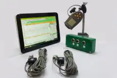
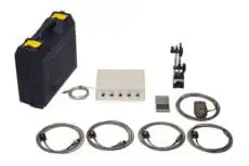
Permanently installed proximity probes feeding a monitoring system are the textbook way to capture an orbit on large critical machines, but the underlying principle — two perpendicular displacement signals plotted against each other with a phase reference — is equally available to the field engineer. A portable two-channel instrument such as the Balanset-1A measures synchronous amplitude and phase on two planes at once, so once an orbit or spectrum has confirmed that unbalance is the dominant force, the same setup carries straight through to field balancing and verification of the corrected state. When the orbit instead reveals misalignment, a rub, or instability, that finding redirects the work toward alignment or a mechanical fix rather than balancing.
Displacement Orbit versus Velocity Orbit
The two are not the same measurement, and the difference decides what you are entitled to conclude from the picture. A pair of proximity probes reads shaft displacement relative to the bearing, so the plot is a true map of where the journal sits inside its clearance, and the DC part of the same signal yields the shaft centreline. A portable two-channel analyser with accelerometers clamped to the bearing housings plots two velocity channels against each other, in mm/s: what you see is the motion of the housing, not the position of the shaft.
What survives the change of transducer is the geometry. Shape, orientation and precession direction are set by the pattern of forces acting on the rotor rather than by the sensor, so the familiar families still appear — a smooth ellipse when 1× dominates, a crescent or figure-8 when a strong 2× component is present, flattened sides and kinks when something rubs. What does not survive is absolute position: a velocity orbit cannot tell you how much clearance is left, and it cannot be rescaled into micrometres of shaft motion. Use it in the field to identify the fault family; reach for proximity probes when the question is where the shaft is actually running.
Where the Orbit Lives in the Balanset Software
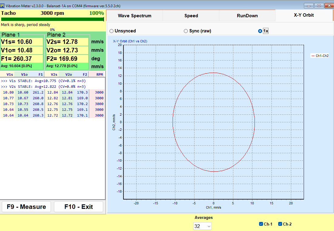
On a Balanset-1A the orbit is one tab of the vibration-meter window, opened with the F5 key from the main window; the window requires device firmware 5.5.0 or newer. The “X-Y Orbit” tab plots channel 1 on one axis against channel 2 on the other at a 1:1 axis scale, so a circle on screen is genuinely a circle and not an artefact of unequal axes. On the four-channel Balanset-4A a second orbit, for channels 3 and 4, is drawn beneath the first.
A switch above the chart decides what is drawn:
| Mode | What is plotted | When it is the right view |
|---|---|---|
| Unsynced | The raw trajectory, with no revolution reference | No tachometer is available, or you want to see everything the signal contains |
| Sync (raw) | The most recent revolutions overlaid, aligned to the tachometer mark | Judging repeatability — a stable, closed figure means the motion repeats turn after turn |
| 1× | The rotational component alone: a clean ellipse that matches the V·o and F readings | Confirming the unbalance vector before balancing |
Without a tachometer mark the two synchronised modes have nothing to synchronise to, the program says so in the chart title, and “Unsynced” becomes the only honest view. This is the practical form of the point made in section 3: no once-per-revolution reference, no precession direction.
Reading the Numbers Beside the Orbit
The tiles next to the chart carry three values per measuring plane, and together they are the fastest sanity check available before you start interpreting shapes:
- V·s — broadband RMS velocity across the working band, in mm/s.
- V·o — the 1× component alone, at rotational frequency, in mm/s.
- F — the phase of that 1× component, in degrees.
The rotational component is part of the total by construction, so V·o can never exceed V·s, and the ratio between them predicts the orbit before you look at it. When V·o sits close to V·s, nearly all the energy is at 1×, the orbit collapses to a clean ellipse, and unbalance is the dominant force. When V·o is markedly smaller, the difference is harmonics and broadband noise — and it is exactly that residue which bends the ellipse into the crescents, figure-8s and kinks described in section 2. A badly distorted orbit reported alongside V·o ≈ V·s is a contradiction, and the instrumentation is the first thing to check.
Beneath each plane sits a stability bar: grey while the reading is still drifting, green once the coefficient of variation over the last twelve stream values falls below 10 %, orange when the spread exceeds 20 %. An orbit captured while that bar is orange is not a diagnosis — it is a photograph of a machine that has not settled.
Confirming the Shape Against the Spectrum
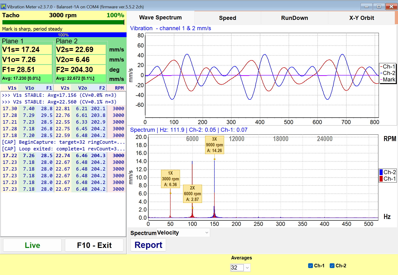
The orbit tells you that something is distorting the ellipse; the spectrum tells you which order is responsible. The “Wave Spectrum” tab of the same window shows the waveform above and the velocity spectrum below, with dashed guides placed at exact multiples of the measured rotational speed rather than at the nearest tall bar — so a peak that misses its marker is not a harmonic of shaft speed at all and belongs to bearings, gear mesh or blade pass instead. A dominant 2× beside a crescent or figure-8 orbit points at misalignment; a peak between 0.43× and 0.48× under a drifting, unstable orbit is the signature of oil whirl; broadband content with flattened orbit sides points at a rub.
The selector below the chart switches the spectrum between velocity and acceleration. Velocity is the axis to use when reasoning about the orbit, because the orbit itself is drawn from the velocity channels.
Watching the Orbit Through a Resonance
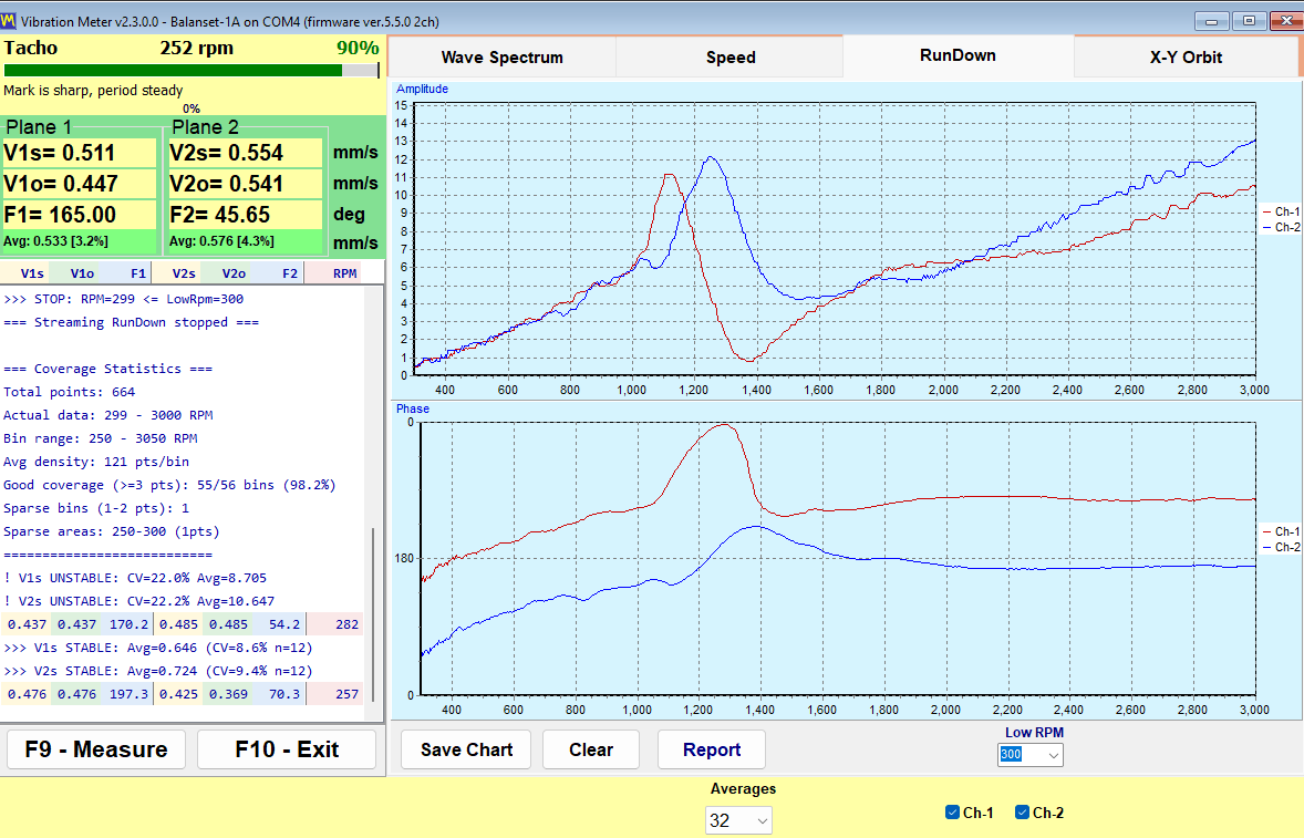
An orbit is a snapshot at one speed, and the shape can change completely a few hundred RPM away. The “Run-down” tab records the whole coast-down instead: 1× amplitude and phase are logged against falling speed, one raw value per revolution with no smoothing, down to a stop threshold that can be set anywhere between 100 and 2000 RPM and defaults to 300. A resonance announces itself as an amplitude peak accompanied by a phase rotation of roughly 180° — the same critical speed that a Campbell diagram predicts where an excitation line crosses a natural-frequency curve. The full run-down report keeps the X-Y orbit captured at working speed alongside those curves, so the shape and the resonance map end up in one document.
5. What an Orbit Plot Shows
In summary, a single orbit plot delivers a wealth of information at a glance:
- The overall amplitude of shaft vibration.
- The shape of the shaft’s motion, which helps identify the fault type.
- The direction of precession, forward or reverse.
- The average position of the shaft within the bearing clearance — its shaft centreline.
Analysed in conjunction with the FFT spectrum and the time waveform, the orbit lets an analyst reach a highly confident and detailed diagnosis of a machine’s dynamic behaviour — combining the “how much,” the “what shape,” and the “which way” into one decisive picture.