了解振動分析中的軸軌跡圖
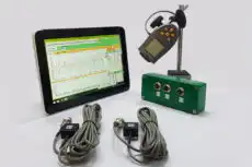

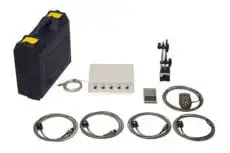

A 軸軌跡 是一種圖表,顯示旋轉軸的幾何中心在一次或多次旋轉期間所繪製的路徑。它是軸在其 軸承游隙內的運動的二维視圖,就像你直視軸的末端一樣。這種強大的診斷方法是通過安裝一對非接觸式 接近感測器 相隔 90 度——通常為 X-Y 配置——並將它們的同時位移信號相互繪製,而不是對時間繪製。
1. 為什麼軌跡圖如此有用
標準的 時域波形 或 FFT 頻譜 顯示 振動 在單一方向上。軌跡圖結合了兩個垂直方向,以提供軸動態運動的完整圖景,讓分析師能夠視覺化運動的實際形狀和方向,而不是推斷它。那個額外的維度為診斷各種故障提供了無價的線索,這就是為什麼軌跡圖是 轉子動力學 分析的基石——特別是對於配備液體薄膜 滑動軸承的高速關鍵機械,如渦輪機、壓縮機和大型發電機。
由於探頭直接相對於軸承測量位移,軌跡圖還揭示了軸在其游隙中的位置,而不僅僅是它移動的距離——這是安裝在機殼上的 加速規 根本無法提供的資訊。添加 轉速計 或 鍵相 標記將每次旋轉印記在軌跡上,固定其 相位 並使進動方向無歧義。
2. 如何解讀軌跡形狀
軌跡的形狀、大小和方向是作用在轉子上的力的直接指標。熟練的分析師通常只需查看軌跡的形狀即可診斷機器的狀況。
圓形或橢圓形軌跡
一個簡單的圓形或橢圓形軌跡,位於軸承中心,通常表示一個行為良好的轉子,由單一頻率主導——最常見的是 不平衡。如果軸承支撐剛性在兩個方向上相同(各向同性),軌跡將是圓形的;如果剛性在水平和垂直方向上不同(各向異性),軌跡將是橢圓形的,這在實踐中非常常見,因為大多數機器在垂直方向上比水平方向更剛硬。
扭曲、數字 8 形或香蕉形軌跡
當軌跡從簡單的橢圓變形時,多個頻率正在影響軸的運動:
- A 「香蕉」形或新月形軌跡 通常與 不對心,其中同時存在 1× 和 2× 頻率。
- A 數字 8 形 是強 2× 組分的經典標誌,是軸不對心的教科書指標。帶有內部環的 8 字形通常表示更嚴重的狀況或存在摩擦。
帶有折角或尖角的軌跡
軌跡中方向的急劇變化、平坦區域或「折角」是 轉子與定子摩擦。這顯示軸的運動,在接觸到固定部件(例如軸承、 密封件或機殼)時,正暫時受到約束。
高度不規則的軌跡
一個不規則、不穩定或看起來充滿「雜訊」的軌跡可能表示嚴重的機械 鬆動、液體誘發的不穩定性,如 油膜渦動 或 油膜振盪,或泵或壓縮機中的湍流條件。
3. 進動方向:順向與逆向
軌跡繪製的方向,相對於軸旋轉的方向,本身就是一個關鍵的診斷因素:
- 正向進動: 軌跡沿著與軸旋轉相同的方向繪製。這是不平衡等力的正常行為。
- 逆向進動: 軌跡沿著與軸旋轉相反的方向繪製。這是一種異常狀況,可能表示 軸裂紋、嚴重摩擦或某些類型的液體誘發不穩定性。
區分這兩者需要每轉一次的相位標記;沒有它,軌跡顯示形狀但不顯示行進方向,診斷區分就會丟失。
4. 現場診斷中的軌跡
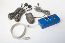
永久安裝的接近探頭連接至監控系統是在大型關鍵機器上捕獲軌跡的教科書方法,但基本原理——兩個垂直位移信號相互繪製並帶有相位參考——同樣適用於現場工程師。像 Balanset-1A 這樣的便攜式雙通道儀器可以同時在兩個平面上測量同步振幅和相位,因此一旦軌跡或頻譜確認 不平衡 是主導力,相同的設置就可以直接進行到 現場動平衡 和校正狀態的驗證。當軌跡反而揭示不對心、摩擦或不穩定性時,該發現會將工作重新導向對中或機械修復,而不是動平衡校正。
位移軌跡與速度軌跡的比較
這兩者並非相同的量測,而這項差異決定了你能從圖形中得出什麼結論。一對接近式感測器讀取的是軸的 位移 相對於軸承的位置,因此該圖是軸頸在其游隙內實際位置的真實地圖,而同一訊號中的直流(DC)成分則產生 軸中心線。而配備加速規並夾附於軸承座上的便攜式雙通道分析儀,則將兩個 速度 通道以 mm/s 為單位相互繪製:你看到的是軸承座外殼的運動,而非軸本身的位置。
更換感測器類型後仍然不變的是幾何形狀。形狀、方向與進動方向是由作用在轉子上的力的模式所決定,而非感測器本身,因此常見的軌跡類型依然會出現——1× 佔主導時呈現平滑橢圓形,存在強烈 2× 成分時呈現新月形或數字 8 形,發生摩擦時則出現扁平邊與折角。無法保留下來的是絕對位置:速度軌跡無法告訴你還剩多少游隙,也無法換算成軸運動的微米數值。在現場可用它來判定故障類型;若要確認軸實際運行的位置,則須改用接近式感測器。
軌跡圖在 Balanset 軟體中的位置
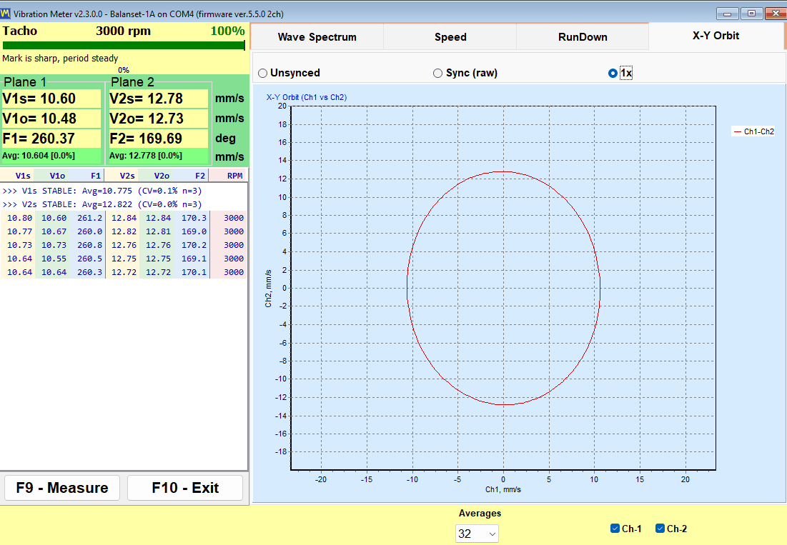
在 Balanset-1A 上,軌跡圖是測振儀視窗中的一個分頁,可從主視窗以 F5 鍵開啟;此視窗需要 5.5.0 或更新版本的裝置韌體。「X-Y Orbit」(X-Y 軌跡)分頁以 1:1 的座標軸比例,將通道 1 與通道 2 相互繪製,因此螢幕上的圓形確實是圓形,而非因座標軸比例不一致所產生的假象。在四通道的 Balanset-4A 上,通道 3 與通道 4 的第二個軌跡會繪製於第一個軌跡下方。
圖表上方的切換開關決定要繪製的內容:
| 模式 | 繪製內容 | 適用情境 |
|---|---|---|
| 未同步 | 原始軌跡,無轉一次參考 | 沒有可用的轉速計,或想查看訊號中包含的所有內容 |
| 同步(原始) | 最近幾轉的軌跡疊加顯示,並對齊轉速計標記 | 判斷重複性——穩定的封閉圖形代表運動每轉皆重複一致 |
| 1× | 僅旋轉分量:呈現與 V·o 及 F 讀數相符的乾淨橢圓形 | 在動平衡校正前確認不平衡向量 |
若沒有轉速計標記,兩種同步模式便無從同步,程式會在圖表標題中如實標示,此時「未同步」就成為唯一誠實的檢視方式。這正是第 3 節所述原則的實務體現:沒有每轉一次參考,就沒有進動方向。
解讀軌跡圖旁的數值
圖表旁的方塊為每個測量平面顯示三個數值,在你開始解讀圖形形狀之前,這三者共同構成最快速的合理性檢查:
- V·s ——工作頻帶內的寬頻 RMS 速度,單位為 mm/s。
- V·o ——僅 1× 分量,即旋轉頻率下的數值,單位為 mm/s。
- F — 這 相位 ,即該 1× 分量的角度,單位為度。
旋轉分量本質上是總量的一部分,因此 V·o 永遠不會超過 V·s,而兩者的比值甚至在你觀察圖形之前就能預測軌跡的形狀。當 V·o 接近 V·s 時,幾乎所有能量都集中在 1×,軌跡會收斂為乾淨的橢圓形,且 不平衡 是主導力。當 V·o 明顯小於 V·s 時,其差值便是諧波與寬頻雜訊——正是這部分殘留能量,將橢圓形扭曲成第 2 節所述的新月形、數字 8 形與折角。若回報嚴重扭曲的軌跡,卻同時顯示 V·o ≈ V·s,則兩者互相矛盾,此時應優先檢查儀器本身。
每個測量平面下方都有一條穩定度指示條:讀數仍在漂移時顯示灰色,最近十二個串流數值的變異係數降至 10% 以下時顯示綠色,離散程度超過 20% 時顯示橙色。若在指示條為橙色時擷取軌跡,並不能作為診斷依據——那只是一台尚未穩定的機器的一張快照。
以頻譜驗證軌跡形狀
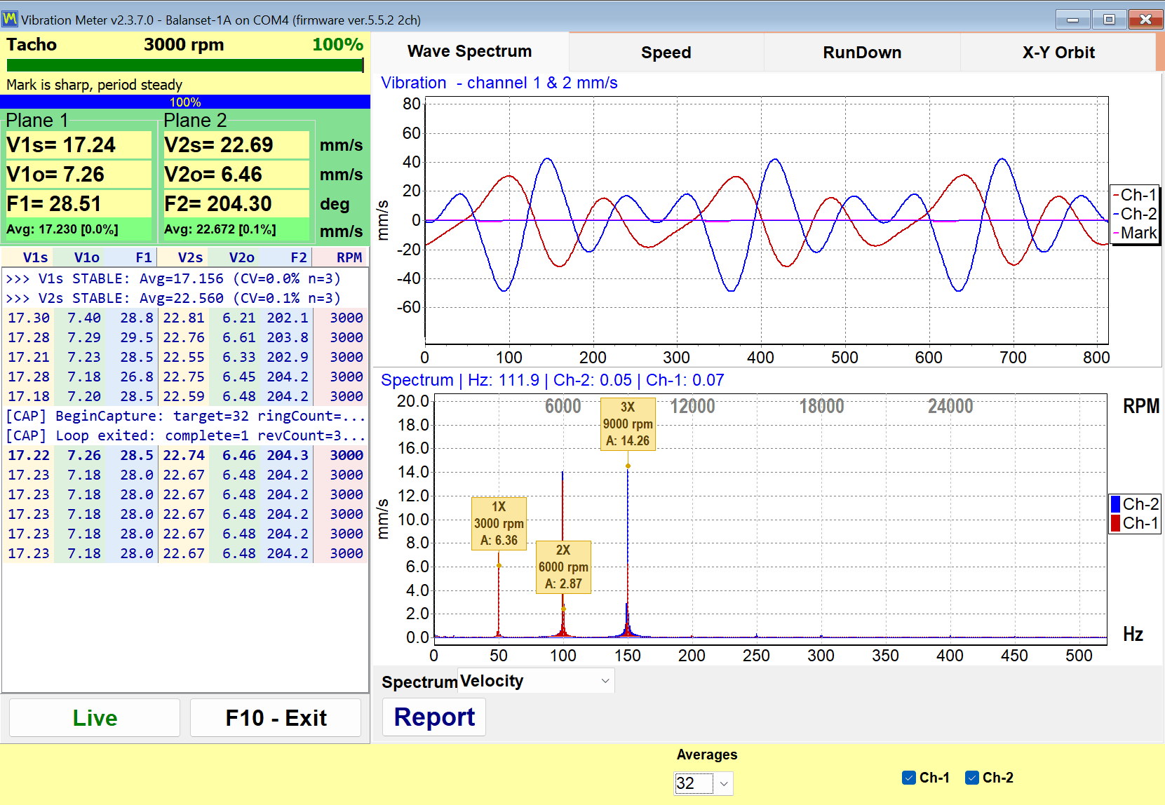
軌跡圖告訴你有某種因素正在扭曲橢圓形;頻譜則告訴你是哪個階次造成的。同一視窗中的「Wave Spectrum」(波形頻譜)分頁,上方顯示波形,下方顯示速度頻譜,虛線標記精確地落在實測轉速的整數倍處,而非落在最接近的高峰上——因此,若某個峰值未對齊標記,就完全不是軸轉速的諧波,而應歸因於軸承、齒輪嚙合或葉片通過頻率。若新月形或數字 8 形軌跡伴隨明顯的 2× 分量,則指向 不對心;若在不穩定、持續漂移的軌跡下出現介於 0.43× 至 0.48× 之間的峰值,則是 油膜渦動的特徵;若寬頻成分伴隨軌跡邊緣變平,則指向 摩擦.
圖表下方的選擇器可在速度與加速度頻譜之間切換。在對照軌跡圖進行分析時,應使用速度軸,因為軌跡圖本身正是由速度通道繪製而成。
觀察軌跡圖如何呈現共振
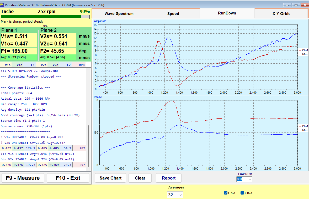
軌跡圖只是某一轉速下的一張快照,形狀可能在僅僅相差數百 RPM 後就完全改變。「Run-down」(降速)分頁則記錄整個惰轉降速過程:1× 振幅與相位會隨轉速下降而逐轉記錄,每轉一個原始數值,不經任何平滑處理,直到可設定於 100 至 2000 RPM 之間、預設為 300 的停止閾值為止。共振會以振幅峰值伴隨約 180° 的相位旋轉來宣告自身——這正是 坎貝爾圖 所預測的、激振線與自然頻率曲線交會處的相同臨界轉速。完整的降速報告會將運轉轉速下擷取的 X-Y 軌跡圖與這些曲線並列保存,讓形狀與共振圖譜最終呈現在同一份文件中。
5. 軌跡圖顯示的內容
總之,單個軌跡圖一瞥即可提供大量資訊:
- 軸振動的總體振幅。
- 軸運動的形狀,有助於識別故障類型。
- 進動方向,順向或逆向。
- 軸在軸承游隙中的平均位置——其 軸中心線.
與 FFT 頻譜和時間波形結合分析,軌跡讓分析師能夠對機器的動態行為做出高度自信且詳細的 診斷 ——將「多少」、「什麼形狀」和「哪個方向」結合到一個決定性的圖景中。