Kuelewa Kusawazisha kwa Tuli (Kusawazisha kwa Uso Mmoja)


Kusawazisha kwa tuli ni aina rahisi zaidi ya rotor kusawazisha. It corrects kusawazishwa kwa statiki — hali ambayo kituo cha wingi cha rotakimezamishwa kutoka kwa mhimili wa mzunguko, linalounda nukta moja ya uzani “nzito.” Kwa sababu nukta hiyo nzito inajionyesha chini ya mvuto tu, urekebishaji unaweza, kwa kanuni, kufanywa na rotor umebaki: weka rotor ulio na uzani safi wa tuli unbalance juu ya uso usio na msuguano kama kingo za kisu, na utazunguka hadi nukta nzito isette chini. Marekebisho yanafanywa katika single plane — uzani mmoja wa marekebisho uliwekwa digrii 180° kinyume cha nukta nzito ili kuleta kituo cha wingi kurudi kwenye kituo cha mzunguko. Urahisi huu wa uso mmoja ndiyo nguvu kubwa ya mbinu na, kama tutakavyoona, pia ni kizuizi chake.
1. Uzani wa Tuli dhidi ya Uzani wa Kigeuzi
Uzani wa tuli pia huitwa “uzani wa nguvu,” kwa sababu inazalisha nguvu ya kituo unayofanya kazi radially nje kutoka kituo cha mzunguko. Muhimu, haizalishi “jozi” au mwendo wa kutulia. Hilo linalifaranisha kutoka kwa kutokuwazimu kwa nguvu, ambayo inachanganya nguvu na kusawazishwa kwa ndani na inahitaji marekebisho katika angalau nyuso mbili kutatua kabisa. Rotor inaweza kusawazishwa kwa ustadi kwa tuli na bado kubeba uzani wa jozi muhimu ambao unalievuta vibrate sana inapozunguka — kwa hiyo sawazishi ya tuli, kwa upande wake, ni inayofaa tu kwa tabaka fulani la rotor.
2. Kusawazisha kwa Tuli Kunatosha Lini?
Kusawazisha kwa tuli kunafaa tu kwa tabaka maalum la rotor. Kwa ujumla huhifadhiwa kwa sehemu ambazo ni nyingi sana au zenye umbo la diski, ambapo urefu wa axial ni ndogo kulinganisha na kipenyo. Kwa rotor kama hizo, uzani wa jozi muhimu hauna uwezekano wa kuwepo mahali pa kwanza, kwa hivyo urekebishaji wa uso mmoja halisi husuluhisha tatizo.
Mifano ya kawaida ambako kusawazisha kwa tuli kwa uso mmoja kunaweza kuwa na kutosha:
- Gurudumu la kusaga
- Gurudumu la motokaa na tairi
- Gurudumu la upepo au na mvuto nyingi na nyingi — leseni
- Flywheels
- Miini na sheaves
Kwa ajili ya rotor yoyote ya urefu mkubwa — armature ya motor, pompa ya hatua nyingi, au shimoni ndefu — kusawazisha tu kwa tuli sio kutosha na kusawazisha kwa nguvu in two planes inahitajika. Mkabala wa uso mmoja yenyewe unafafanuliwa zaidi chini ya usawazishaji wa uso mmoja.
3. Njia za Kusawazisha Tuli
1. Kusawazisha kwa Upinde wa Kisu
Hii ndio njia ya kawaida, isiyo na kuzunguka. Rotor huwekwa kwenye jozi ya upinde sambamba, ulio uwazi, wenye uvimbe mdogo. Inalegeza hadi hatua yake nzito sana iwe chini; kiwango cha muda kinaweza kuongezwa kwenye juu (180° kinyume) hadi rotor itakamatia bila kulegeza. Kiwango hicho kinafanywa daima. Haitaji nguvu na haitaji umeme — tu subira na jozi ya upinde wa kweli, uwazi — na inabaki kuwa njia halisi ya ukaguzi wa mahali kwa diski nyingi.
2. Mashine ya Kusawazisha Wima
Kusawazisha kwa tuli kwa sasa mara nyingi hufanyika kwenye mashine ya kusawazisha. Rotor — gurudumu la ndoto au tairi, kwa mfano — inakamatia kwenye sahani ya usawa iliyoungwa na sensorer za nguvu. Mashine huizunguza kwa kasi ndogo, na sensorer hupimia ukubwa na mwelekeo wa nguvu ya kusawazisha, ikicheza matokeo yanayohitajika kwenye skrini. Kwa ajili ya gurudumu na tairi tu, a calculator ya uzani wa kusawazisha gurudumu hubadilisha usomaji huo kuwa kuku au uzani wa adhesive.
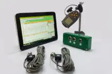
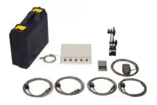
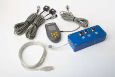
3. Kusawazisha kwa Uso Mmoja wa Mahali (Balanset-1A)
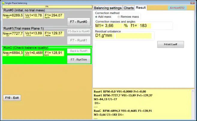
Kusawazisha kwa tuli (uso mmoja) kunaweza pia kufanywa kwenye mashine iliyojengwa kabisa kwa kutumia mfumo wa kusawazisha wa kuhamia — kiini cha field balancing. With the Balancet-1A, hali ya “Kusawazisha kwenye uso mmoja (‘tuli’)” hupima kasi ya rotor (RPM) na vekta ya 1× vibration — its RMS value and phase. Kutoka kwa kiwango cha “Kuendesha #0” na “Kuendesha #1”, programu huhesabu kiotomatiki mass and pembe ya kupanga ya uzani wa kurekebisha unaokamatia kupunguza kusawazisha kwa rotor, kwa kutumia influence-coefficient method.
Matokeo ya kusawazisha ynahifadhiwa kwenye kumbukumbu, na kumaliziwa a ripoti ya kusawazisha zinaweza kuzalishwa, kuhariri, na kupigia chapa katika mhariri wa ripoti iliyojengewa ndani.
Jinsi ambavyo uzani wa uso mmoja unafanywa katika programu ya Balanset-1A
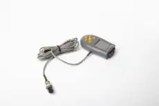
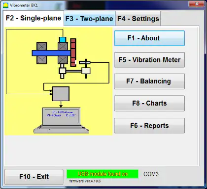
- Sakinisha sensorer na kuunganisha mfumo. Sakinisha sensorer ya mitetemo katika kituo cha kipimo kilichochaguliwa na kuiunganisha kwa kifaa. Sakinisha sensorer ya awamu ("tachometer), apply bendera inayoakisi kwenye rotor, na kuunganisha kifaa kwa kompyuta ya Windows.
- Anza hali ya Uzani wa Uso Mmoja. Katika dirisha la shughuli kuu chagua hali ya “uzani wa uso mmoja” na anza uzani. Programu inafungua dirisha la faili la uzani wa uso mmoja.
- Tengeneza rekodi ya faili. Ingiza jina la rotor, mahali pa kusakinisha, vikomo (vibration na sawa na juu-juu ndogo), na tarehe. Programu inatengeneza folda ya faili ambapo chati na faili za ripoti zitahifadhiwa.
- Teua vigezo vya uzani katika “mipango ya uzani”.
- Mgawo wa ushawishi: chagua “Rotor Mpya” (mbio mbili kukadiria) au “mgawo umefadhiliwa” (mbio moja, kwa aina sawa ya mashine yenye migawo ya ushawishi iliyohifadhiwa).
- Uzani wa uzani wa jaribu: chagua “Gramu” au “Asilimia”. Ikiwa unatarajia kutumia hali ya “mgawo umefadhiliwa” baadaye, ingiza trial weight uzani kwa gramu (kupima kwa kiwimbi).
- Njia ya Kusambaza Uzani: chagua “Zingira” (pembe yoyote kwenye mzunguko) au “Mahali pamoja” (mashimo/matawi/nafasi iliyosambazwa; ingiza idadi ya nafasi).
- Radi ya kusambaza uzani: ingiza radi inayotumiwa kwa kusambaza uzani wa jaribio na uamuzi.
- Acha uzani wa mtihani katika Kiwanja 1: Wezesha hili tu ikiwa huwezi kuondoa uzani wa mtihani wakati wa mchakato.
- Mbio #0 (mbio ya awali, hakuna uzani wa mtihani). Leta mashine kwa kasi thabiti na anza “Mbio #0” kupima mitetemo ya awali. Programu inarekodia RPM, thamani ya RMS na awamu ya sehemu ya mitetemo ya 1×. Kichupo cha “Chati” kinaonyesha wimbi na spektramu.
- Sakinisha uzani wa mtihani. Simamisha mashine na sakinisha uzani wa mtihani katika radius inayojulikana. Uzani wa mtihani lazima ubadilishe amplitude au awamu ya mitetemo kwa kiasi kikubwa. Kaida ya kawaida ni “sheria ya 30/30”: uzani wa mtihani unapaswa kubadilisha amplitude kwa kawaida 30% (chini au juu) au awamu kwa kawaida 30° au zaidi. Ikiwa unapanga kutumia hali ya “Mgawo uliohifadhiwa” baadaye, sakinisha uzani wa mtihani katika pembe sawa na alama ya kuakisi.
- Mbio #1 (uzani wa mtihani umesakinishwa). Anzisha upya mashine, subiri kasi thabiti, na fanya “Mbio #1”. Programu inahesabu vigezo vya uzani wa kusambaza.
- Sakinisha uzani wa kusambaza. Simamisha mashine, ondoa uzani wa mtihani, na sakinisha uzani wa kurekebisho. Pembe ya usakinishaji inahesabiwa kutoka kwa nafasi ya uzani wa mtihani katika mwelekeo wa mzunguko wa rotor. Sakinisha uzani wa kusambaza katika radius sawa na uzani wa mtihani.
- RunTrim (angalia ubora wa usawazaji). Fanya “RunTrim” kuangalia matokeo. Ikiwa mitetemo yaliyosalia na/au kutokuwa na usawa maalum kukidhi toleransi, usawazaji unaweza kukamilika. Ikiwa sivyo, programu inahesabu uzani wa kusambaza kwa ziada na usawazaji unaendelea kwa makadirio ya mfuatano.
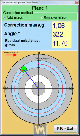
Taswira ya matokeo: grafu ya polar na nafasi zilizowekwa
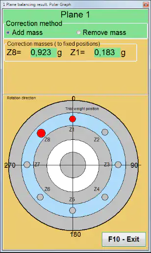
Balanset-1A inaweza kuonyesha uzani na pembe ya uzani wa kusambaza katika mwonekano wa kuratibu cha polar. Ikiwa “Nafasi iliyowekwa” imechaguliwa, programu inaweza kugawanya uzani wa kusambaza kiotomatiki katika sehemu mbili na kuonyesha namba za nafasi ambapo kila sehemu lazima isambazwe — uzuri unaofikiwa na kikokotoo cha kusambaza baledi kwa ajili ya wanamakali na impela zilizo na alama za kumweka zilizosimama.
4. Kuthibitisha Matokeo Dhidi ya Uvumiliano
Usawa wa tuli umekamilika tu wakati vibration ya baki na unbalance ya baki vinaanguka ndani ya uvumiliano unaokubali, ambao ni mahali ambapo hatua ya RunTrim inaonyesha thamani yake. Unbalance ya baki inayokubalika kawaida huchorwa kutoka kwa ubora wa usawa G-grade chini ya ya mtazamo ISO 21940-11 kiwango cha ISO (ambacho kilichambulia kiwango cha zamani cha ISO 1940-1). Kubadilisha daraja la G na kasi ya huduma kuwa takwimu yenye gramu-milimita inayokubalika — na kuchagua uzani wa mtihani wa mwanzo wenye akili — ni haraka kwa kikokotoo cha unbalance ya baki (ISO 21940-11) and a kikokotoo cha uzani wa kujaribu. Kurekodi unbalance ya baki wa mwanzo na wa mwisho unakupa kipimo halisi cha jinsi kazi ilitumia au ilifaulu na kuunda msingi wa ripoti ya kulazimisha.
5. Limitations
Kikwazo kuu cha kulazimisha kwa tuli ni ketidza yake ya kutambua au kusahihisha unbalance ya jozi. Kutumia usawa wa tuli kwa rotor ambayo kwa kweli ina unbalance ya nguvu inaweza wakati mwingine kusambaza mambo mengi — kusahihisha sehemu ya nguvu huku ukaingia au hata kuharibika, sehemu ya jozi. Kwa sababu hii, kwa jengo la makina ya viwanda vingi, kulazimisha kwa nguvu kwa pande mbili ndilo kiwango na jambo linalohitajika, na usawa wa tuli ni bora kuhifadhiwa kwa rotor nyembamba zenye umbo la diski ambapo dhana yake ya pande moja kwa kweli inabaki.
