傅立葉變換在振動訊號分析中的應用
Andrei Shelkovenko。Vibromera 的開發者與創辦人之一。
本文翻譯可能含有不準確之處。
傅立葉變換與訊號頻譜
在許多情況下,獲取(計算) 頻譜 訊號的任務如下。有一個 ADC,它以採樣 頻率 Fd 將時長為 T 內輸入其端子的連續訊號轉換為數位樣本 – N 個。然後將這組樣本輸入某個程式(例如 FourierScope)該程式會輸出 N/2 個數值。
為了檢查程式是否正常運作,我們構建一個由兩個正弦函數相加而成的樣本陣列 sin(10*2*pi*x)+0.5*sin(5*2*pi*x) 並輸入程式。程式繪製出以下結果:
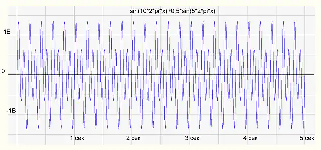
圖 1 訊號時間函數圖
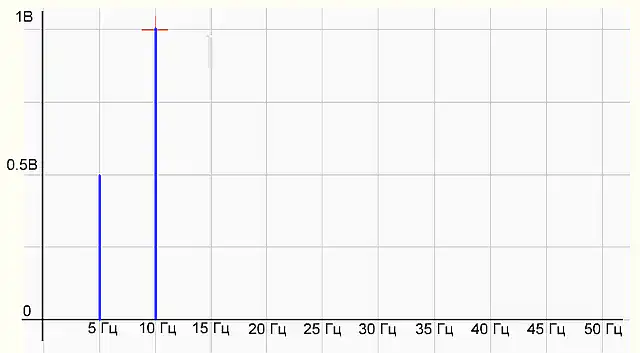
圖 2 訊號頻譜圖
有兩個 諧波 在頻譜圖上 – 5 Hz 振幅為 0.5 V,10 Hz 振幅為 1 V,一切與原始訊號公式中的情況一致。沒問題,程式運作正確。
這意味著,如果我們將由兩個正弦波混合而成的真實訊號輸入 ADC,我們將獲得一個由兩個諧波組成的類似頻譜。
因此,我們的 真實 測量訊號 持續時間為 5 秒,經 ADC 數位化,即表示為 離散 樣本,具有 離散非週期性 頻譜。
從數學角度來看 – 這句話有多少處錯誤?
現在讓我們嘗試測量同一訊號,持續時間為 0.5 秒。
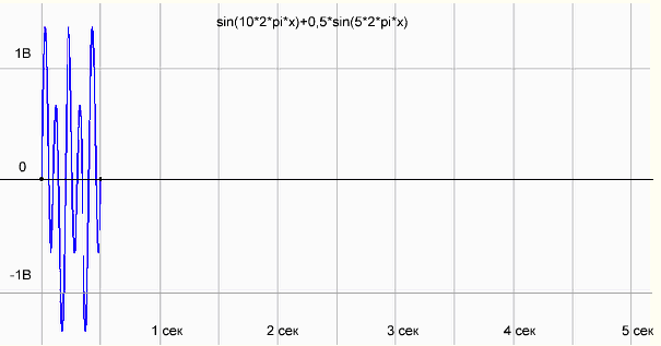
圖 3 測量週期為 0.5 秒的函數 sin(10*2*pi*x)+0.5*sin(5*2*pi*x) 圖
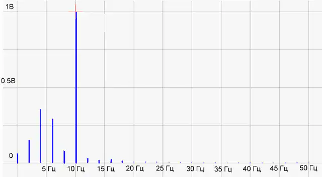
圖 4 該函數的頻譜
這裡有些問題!10 Hz 的諧波繪製正常,但 5 Hz 的諧波位置出現了一些不明確的諧波。
網路上說需要在樣本末尾補零,頻譜就會正常繪製。
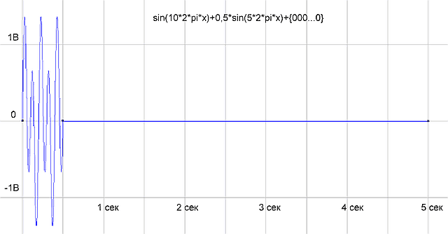
圖 5 我們已在樣本末尾補零至 5 秒
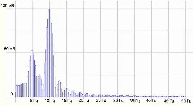
圖 6. 獲得的頻譜。
這完全不是那麼回事。我必須深入研究理論。讓我們前往 wikipedia – 知識的來源。
連續函數及其傅立葉級數表示
從數學角度來看,我們持續時間為 T 秒的訊號是定義在區間 {0, T} 上的某個函數 f(x)(此處 X 為時間)。此類函數總可以表示為以下形式的諧波函數(正弦或餘弦)之和:

(1),其中:
k 為三角函數的序數(諧波分量的序數,諧波的序數)
T – 函數定義的區間(訊號的持續時間)
Ak- 第 k 個諧波分量的振幅,
θk- 第 k 個諧波分量的初始相位
「將函數表示為級數之和」是什麼意思?這意味著,通過在每個點上將傅立葉級數的諧波分量值相加,我們得到該點上我們函數的值。
(更嚴格地說,級數與函數 f(x) 的均方偏差將趨於零,但儘管存在均方收斂,一般而言,函數的傅立葉級數不一定逐點收斂於該函數。)
此級數也可以寫成以下形式:
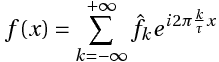
(2),
其中  ,第 k 個複振幅。
或

(3)
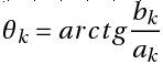
係數(1)與(3)之間的關係由以下公式表示:
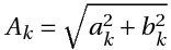
注意,傅立葉級數的這三種表示法完全等效。有時在處理傅立葉級數時,使用虛數參數的指數而非弦波與餘弦波(即使用複數形式的傅立葉變換)會更方便。但對我們而言,使用公式 (1) 更為方便,其中傅立葉級數表示為具有對應振幅與相位的餘弦波之和。嚴格來說,真實訊號的傅立葉變換確實會產生複數係數(形式 (3)):每個係數同時攜帶其諧波的振幅與相位。對於真實訊號,這些複數係數具有共軛(厄米特)對稱性 – 負頻率半部單純是正頻率半部的鏡像,且不攜帶額外資訊。因此,從複數係數中,我們總能轉換至公式 (1) 的實數非負振幅 Ak 與相位 θk – 而分析程式繪製的正是此振幅頻譜。
總結:
訊號頻譜分析的數學基礎是傅立葉變換。
傅立葉變換允許將定義在區間 {0, T} 上的連續函數 f(x)(訊號)表示為無窮多個(無窮級數)具有確定振幅和相位的三角函數(正弦和/或餘弦)之和,這些三角函數同樣考慮在區間 {0, T} 上。此類級數稱為傅立葉級數。
請注意更多要點,理解這些要點對於正確將傅立葉變換應用於訊號分析是必需的。如果我們在整個 X 軸上考慮傅立葉級數(正弦波之和),我們會發現,在區間 {0, T} 之外,傅立葉級數函數將週期性地重複我們的函數。
例如,在圖 7 的圖表中,原始函數定義在區間 {-T\2, +T\2} 上,而傅立葉級數表示定義在整個 x 軸上的週期函數。
這是因為正弦波本身就是週期函數,因此它們的總和也會是週期函數。
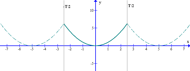
圖 7 以傅立葉級數表示非週期性原始函數
因此:
我們的原始函數是定義在長度為 T 的某區段上的連續非週期函數。
此函數的頻譜是離散的,亦即以無限個諧波分量組成的級數——傅立葉級數——來表示。
實際上,傅立葉級數定義的是某個週期函數,該函數在區間{0, T}上與我們的函數重合,但對我們而言,這種週期性並非關鍵所在。
下一步。
諧波分量的週期是區間 {0, T} 的倍數,初始函數 f(x) 即定義在此區間上。換言之,諧波的週期是訊號量測持續時間的倍數。例如,傅立葉級數中第一諧波的週期等於函數 f(x) 所定義的區間 T。第二諧波的週期等於 T/2,依此類推(見圖 8)。
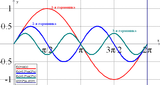
圖8 傅立葉級數諧波分量的週期(頻率)(此處T=2π)
因此,諧波分量的頻率為 1/T 的整數倍。也就是說,諧波分量的頻率 Fk 為 Fk= k\T,其中 k 的取值範圍為 0 至 ∞,例如:k=0 時 F0=0;k=1 時 F1=1\T;k=2 時 F2=2\T;k=3 時 F3=3\T;…。Fk= k\T(頻率為零時,即為直流分量)。
假設我們的初始函數是在 T=1 秒內記錄的訊號。那麼第一諧波的週期將等於訊號的持續時間 T1=T=1 秒,其頻率為 1 Hz。第二諧波的週期將等於訊號持續時間除以 2(T2=T/2=0.5 秒),其頻率為 2 Hz。第三諧波則為 T3=T/3 秒,頻率為 3 Hz。依此類推。
本例中諧波之間的間距為1 Hz。
因此,持續時間為 1 秒的訊號可分解為諧波分量(以取得頻譜),其頻率解析度為 1 Hz。
若要將解析度提高 2 倍至 0.5 Hz,則必須將測量時長提高 2 倍至 2 秒。10 秒的訊號可分解為頻率解析度為 0.1 Hz 的諧波分量(頻譜)。沒有其他方法可提高頻率解析度。您可以透過我們的 FFT 解析度計算器.
有一種方法可以透過在取樣陣列中補零來人為延長訊號時長,但這並不會提升真實的頻率解析度。
離散訊號與離散傅立葉變換
隨著數位技術的發展,量測數據(訊號)的儲存方式也隨之改變。過去訊號可以用磁帶錄音機記錄,以類比形式儲存在磁帶上;而現在訊號則被數位化,並以一組數字(採樣點)的形式儲存在電腦記憶體的檔案中。
訊號測量與數位化的一般流程如下所示。
測量感測器 —- 訊號調理器 —- ADC —– 電腦
(圖9 測量通道示意圖)
來自測量傳感器的訊號會在時間T內送入類比數位轉換器(ADC)。在時間T內取得的訊號讀數(取樣值)會被傳送至電腦並儲存於記憶體中。
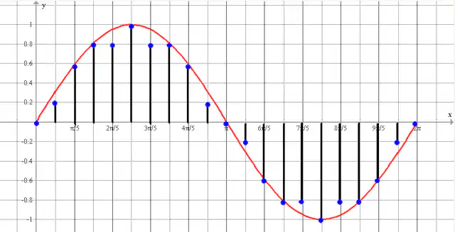
圖10 數位化訊號 – 在時間 T 內取得 N 個取樣點
訊號數位化參數有哪些要求?將輸入類比訊號轉換為離散代碼(數位訊號)的裝置稱為類比數位轉換器(ADC)(© Wiki)。
類比數位轉換器(ADC)的基本參數之一是最大取樣率——即對時間上連續的訊號進行取樣的頻率。取樣率以赫茲為單位。((© Wiki))
根據科捷爾尼科夫定理,若連續訊號的頻譜受限於頻率 Fmax,則可從以時間間隔 Δt ≤ 1/(2*Fmax)(即採樣頻率 Fd ≥ 2*Fmax)取得的離散樣本中完整且唯一地重建該訊號,其中 Fd – 採樣頻率;Fmax – 訊號頻譜的最大頻率。換言之,訊號數位化的頻率(ADC 的採樣頻率)必須至少為我們欲測量訊號最大頻率的兩倍。
那麼,如果我們以低於科捷利尼科夫定理(Kotelnikov's theorem)所要求的頻率進行採樣,會發生什麼情況呢?
在這種情況下存在「混疊」效應(亦稱頻閃效應、莫爾效應),其中高頻訊號在數位化後轉變為實際上並不存在低頻訊號。在圖 11 中,紅色高頻弦波為真實訊號。藍色低頻弦波為虛構訊號,其產生原因是採樣時間內已超過高頻訊號的一半週期。
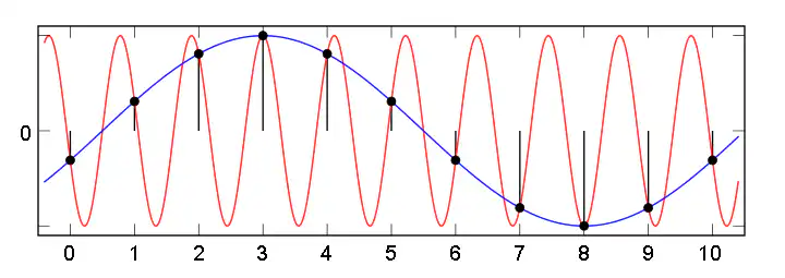
圖 11.在取樣率不足時出現的虛假低頻訊號
為避免混疊效應,會在 ADC 之前放置特殊的抗混疊濾波器(低通濾波器)。它允許低於 ADC 採樣頻率一半的頻率通過,並切斷更高的頻率。
為了根據離散樣本計算訊號頻譜,需使用離散 傅立葉變換(DFT) 。再次注意,離散訊號的頻譜「根據定義」受限於小於採樣頻率 Fd 一半的頻率 Fmax。因此,離散訊號的頻譜可表示為 一個有限的 諧波數量有限,這與連續訊號的傅立葉級數(其頻譜可以是無限的)之無窮總和不同。根據科捷利尼科夫定理,諧波的最高頻率必須至少對應兩個採樣點,因此諧波數量等於離散訊號採樣點數的一半。也就是說,若採樣中有 N 個採樣點,則頻譜中的諧波數量將為 N/2。
現在來看離散傅立葉變換(DFT)。
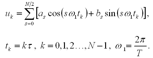
將其與傅立葉級數比較
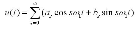
如我們所見,兩者是一致的,唯一的區別在於 FFT 中的時間是離散的,且諧波數量被限制為 N/2,即採樣點數的一半。
離散傅立葉變換(DFT)公式以無因次的整數變數k、s表示,其中k為訊號取樣點數,s為頻譜分量數。
數值 s 代表每個週期 T(訊號測量時長)內完整諧波振盪的次數。離散傅立葉變換用於以數值方式(即「在電腦上」)求得各諧波的幅值與相位。
如前所述,當將非週期函數(我們的訊號)分解為傅立葉級數時,所得到的傅立葉級數實際上對應於一個週期為 T 的週期函數(圖12)。
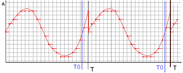
圖12。週期為T0的週期函數f(x),其週期T>T0
如圖 12 所示,函數 f(x) 為週期為 T0 的週期函數。然而,由於測量樣本長度 T 不等於函數週期 T0,作為傅立葉級數獲得的函數在 T 點處存在不連續性。結果,該函數的頻譜將包含大量高頻諧波。此現象稱為 頻譜洩漏,在實務上可透過 加窗 變換前的訊號來減少。若測量樣本時長 T 與函數週期 T0 重合,則傅立葉變換後獲得的頻譜將僅包含第一諧波(週期等於樣本時長的弦波),因為函數 f(x) 為弦波。
換句話說,DFT 程式「並不知道」我們的訊號是「正弦波的一個片段」,而是試圖用級數來表示一個週期函數,該函數因各段正弦波之間的不連續而存在間斷。
因此,頻譜中會出現諧波,這些諧波整體上應能呈現該函數的形狀,包括其中的不連續點。
因此,若要得到由多個不同週期正弦波疊加而成之訊號的「正確」頻譜,就必須使 整數個週期的 每個正弦分量都應存在於訊號的測量週期內。在實務上,只要訊號測量時長足夠長,即可滿足此條件。
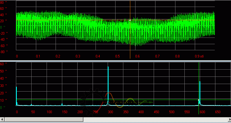
圖 13 齒輪箱運動誤差訊號函數與頻譜範例
若持續時間較短,畫面看起來會「較差」:
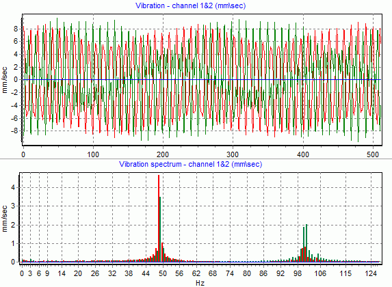
圖 14 轉子振動函數與頻譜範例
在實務中,往往很難分辨哪些是“真實成分”,哪些是由於分量週期與訊號取樣時長不一致,或波形中出現“跳變與斷點”所造成的“偽像”。當然,“真實成分”與“偽像”這兩個詞之所以加上引號,是有原因的。頻譜圖上出現許多諧波,並不代表我們的訊號實際上就是由這些諧波組成的。這就好比認為數字7是由數字3和4“組成”一樣。可以說數字7是3與4之和–這是正確的。
所以我們的訊號……更確切地說,並非「我們的訊號」,而是由我們的訊號(樣本)重複而構成的週期函數,可以表示為若干具有特定振幅與相位的諧波(正弦波)之和。但在許多對實務很重要的情況下(見上圖),確實可以將頻譜中得到的諧波,與具有週期性且對訊號形狀有顯著貢獻的實際過程聯繫起來。
部分結果
1. 經 ADC 數位化、時長為 T 秒的實際測量訊號,即由一組離散樣本(N 個)表示,其頻譜為離散非週期性,由一組諧波分量(N/2 個)表示。
2. 訊號由一組實數值表示。其 DFT 頻譜為一組具有共軛對稱性的複數係數;由此可獲得振幅頻譜 – 即正頻率處的實數非負振幅(與相位)集合,而實務上繪製的正是此單邊振幅頻譜。包含負頻率的雙邊複數形式與單邊振幅/相位形式為同一頻譜的等效表示 – 對於訊號分析而言,通常使用單邊振幅頻譜更為方便。
3. 在時間 T 內測量的訊號僅在時間 T 內被確定。在我們開始測量訊號之前發生了什麼,以及之後會發生什麼,科學上並不知道。而在我們的情況下,這也不重要。有限時間訊號的 FFT 給出了其「真實」頻譜,意即在特定條件下,它允許計算其分量的振幅與頻率。

Nikolai Shelkovenko
Nikolai Shelkovenko是一名振動分析工程師,也是Vibromera的創辦人兼執行長。 15年多來,他一直在現場——而非在試驗台上——為旋轉設備進行動平衡校正:粉碎機、工業風機、破碎機、離心機、軸與主軸。正是這些實際工作催生了Balanset系列儀器——它們被設計為一種專業人員可以隨身攜帶到機器旁、在現場獨立使用的工具,而非實驗室設備。 Vibromera成立於2017年,自2023年起總部設於葡萄牙波爾圖。Balanset系列產品的研發、組裝與支援均在此完成。旗艦產品是Balanset-1A,一款用於單平面及雙平面動平衡校正與振動診斷的可攜式分析儀。 Nikolai親自參與客戶支援工作,處理各種棘手的動平衡校正案例,並參與軟體開發。他以任何語言為全球客戶提供服務。