Every Balanset-1A and Balanset-4A ships with the same Windows program, which is a vibration meter, an FFT analyser and a field balancing calculator in one application. It measures overall RMS in mm/s, the 1x component with amplitude and phase, RPM, spectrum, waveform, shaft orbit and run-down, then calculates correction weights for 1 to 4 correction planes from your own trial runs and checks the residual unbalance against ISO 1940. The program runs locally on Windows 7 through Windows 11, reads the instrument over a USB COM port, and needs no internet connection, cloud account or subscription.
What the Balanset software is, and who uses it
The Balanset program is a single Windows application that does two jobs with the same instrument and the same sensors. It measures machine vibration: overall RMS level, the 1x rotational component with amplitude and phase, RPM, spectrum, waveform, shaft orbit and run-down. It also performs dynamic balancing of rotors in their own bearings, in 1, 2, 3 or 4 correction planes, calculating the correction weight from your own trial runs on your own machine. Diagnosis and repair therefore happen in one session, at the machine, without exporting data to a second tool.
The program is written for maintenance and service engineers who balance rotors on site: fans, blowers, impellers, crushers, augers, centrifuges, turbines, grinding wheels and drive shafts. The rotor stays in its own bearings and is not dismounted, and the machine is balanced at its normal operating speed, which is the condition it actually runs in.
It is an ordinary local Windows application, not a web service. There is no cloud, no account and no subscription, and the instrument is read over a USB COM port. A field laptop with no network connection at all is a complete working setup.
The software is included with the instrument. Balanset-1A costs €1,975 and Balanset-4A costs €6,803. Specifications and ordering are on the Balanset-1A product page and the Balanset-4A product page, and a pre-sales question can be sent to us on WhatsApp.
One program, two instruments
The same program serves both instruments and recognises which one is plugged in. It reads the channel count from the firmware and hides Ch-3 and Ch-4 when they do not physically exist, so the interface never offers a measurement the hardware cannot make.
| Instrument | Vibration channels | Tacho channel | Maximum correction planes | Price |
|---|---|---|---|---|
| Balanset-1A | 2 (Ch-1, Ch-2) | 1 | 2 | €1,975 |
| Balanset-4A | 4 (Ch-1 to Ch-4) | 1 | 4 | €6,803 |
The maximum number of correction planes equals the number of vibration channels. Three and four planes are available only on the 4-channel Balanset-4A and only in the Modern balancing form; on Balanset-1A the maximum is two planes.
Firmware 5.5.0 or newer is required
This belongs at the top of the page rather than in a footnote, because it decides whether the program will measure at all. This version of the software measures only with instrument firmware 5.5.0 or newer. On firmware 4.10.x, and on the intermediate versions 5.0.x to 5.4.x, the device is still detected and its COM port is still visible, but no measurement will start and the connection line reads “Firmware not supported on COMx”. The firmware itself is updated from the program, from the “Updates” window.
Connection, keyboard and colour coding
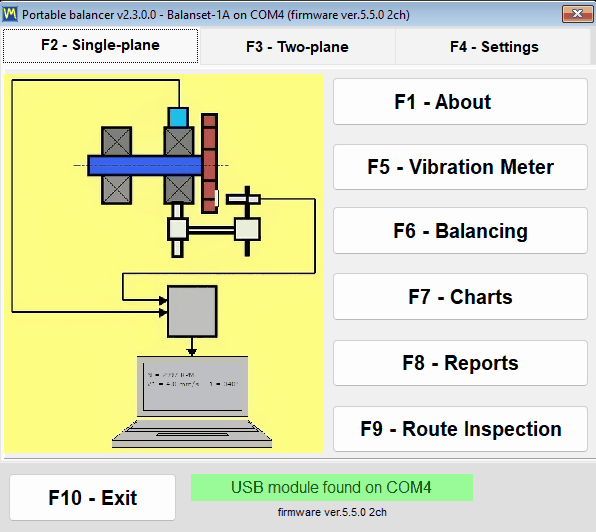
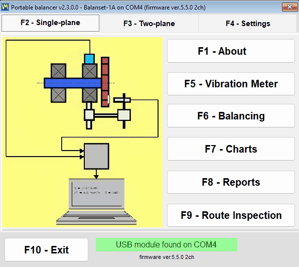
There is no Connect button anywhere in the program. It scans the COM ports about every 1.5 seconds and picks up the instrument at any moment, including hot-plug while a measurement window is already open. The model, the COM port and the firmware version are shown in the window title, so you always know what you are talking to.

The whole program can be driven from the keyboard, F1 to F10, and F12 saves a PNG screenshot of the current window into Documents\Bs1A\Screenshots. On a field laptop, with one hand on the machine and no mouse surface anywhere nearby, that is the difference between recording a result and losing it.
Channel colour coding is consistent across every chart, table and report, so a colour in a printed protocol means the same thing as on screen:
- Ch-1 is dark red.
- Ch-2 is blue.
- Ch-3 is green.
- Ch-4 is amber.
- Tacho is magenta.
Vibration Meter: live readings, run-down and shaft orbit
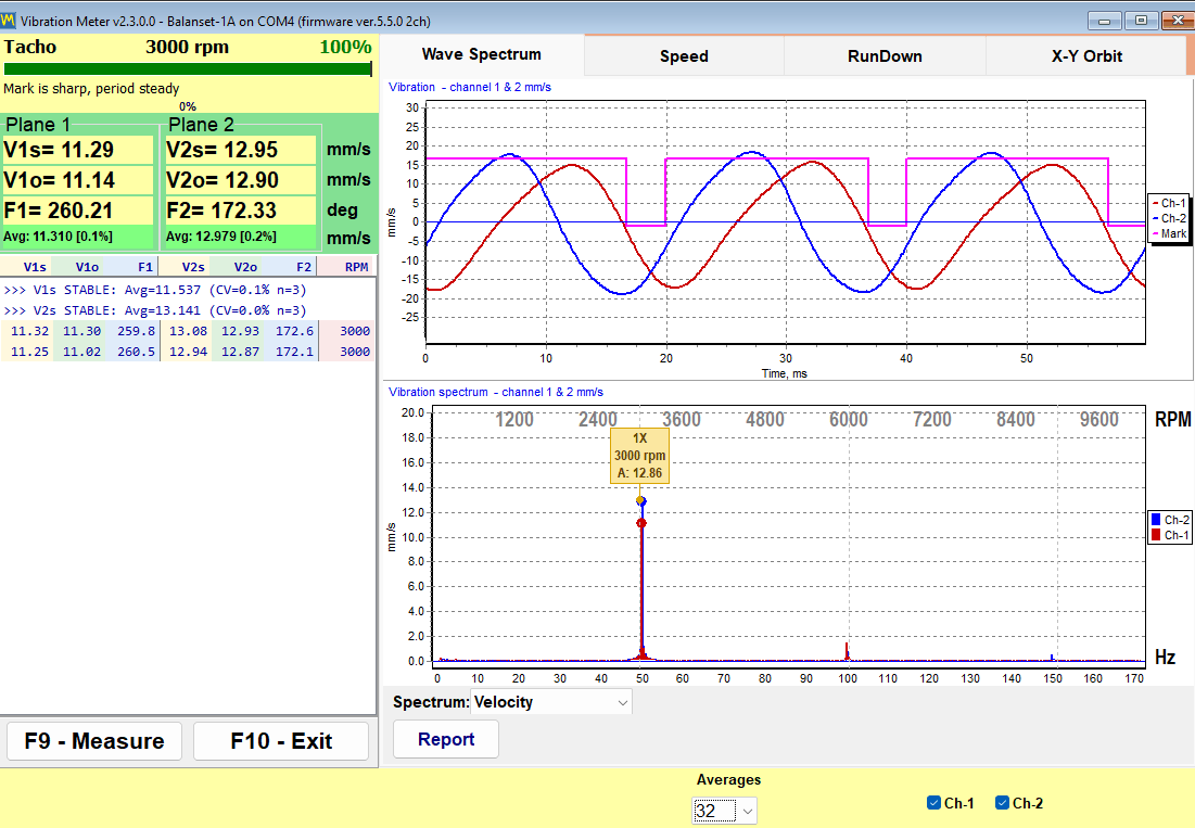
Before it is a balancer, the product is a working vibration meter. The Vibration Meter window streams every channel at once and keeps the values on screen while you move a sensor, change the speed or wait for a machine to settle. For each channel it shows four numbers, where the asterisk stands for the channel number.
| Readout | What it is |
|---|---|
| V*s | Overall RMS vibration velocity in the working band, in mm/s. |
| V*o | The 1x component, that is the part of the vibration occurring at rotational frequency, in mm/s. |
| F* | The phase of that 1x component, in degrees, referenced to the tacho mark. |
| RPM | Rotational speed measured by the laser tacho sensor. |
Six tabs sit inside the meter:
- “Wave” shows the time waveform.
- “Spectrum” shows the FFT spectrum, either as velocity in mm/s or as acceleration in m/s2.
- “Speed” shows the rotational speed over time.
- “Run-down” records 1x amplitude and phase against falling RPM during a coast-down.
- “X-Y Orbit” draws the path of the shaft from two channels.
- “Bump test” finds natural frequencies from a hammer strike, and is experimental and off by default.
A stability indicator tells the operator when a reading can be trusted. The program watches the scatter of the recent values and reports STABLE when the coefficient of variation stays under 10 percent on two consecutive evaluations, and UNSTABLE when it goes above 20 percent. A signal below 0.005 mm/s is treated as no signal rather than as a very small one. This is the practical difference between writing down a measurement and writing down noise.
F9 freezes the current measurement so that it can be read, compared with the next one and placed into a report while the machine is still running. Charts export to BMP or WMF when a document has to be assembled somewhere else.
Run-down: find the resonances before you balance
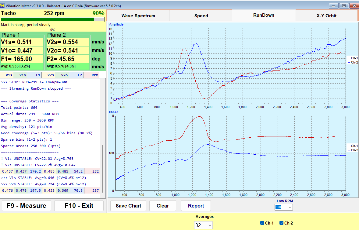
A run-down is recorded by bringing the rotor up to speed, switching the drive off and letting it coast. The program records the 1x amplitude and phase against the falling RPM and stops by itself at the “Low RPM” threshold, which is adjustable from 100 to 2000 and defaults to 300. A resonance shows up as a peak in amplitude together with a phase reversal of roughly 180 degrees, and it is that pair of signs together, not the peak alone, that identifies a resonance.
This is the cheapest test on the whole page in commercial terms. Balancing near a support resonance is unreliable, because the amplitude is amplified and the phase drifts, so a job that refuses to converge after several trial runs is often a machine running close to a critical speed. Two minutes of coast-down before the job tells you that, and saves the wasted runs.
X-Y Orbit: the shape of the shaft motion
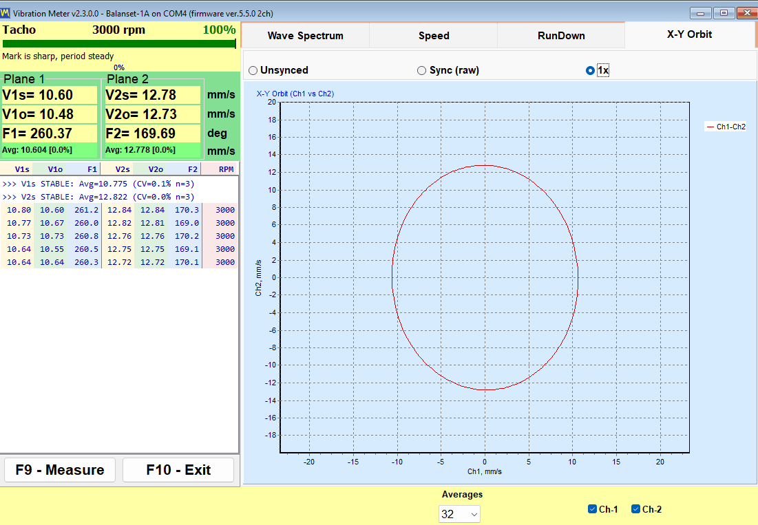
X-Y Orbit plots the path of the shaft from two channels on a 1:1 axis scale, so the shape is not distorted by the scaling. Three modes are available: “Unsynced”, “Sync (raw)” and “1x”. On Balanset-4A, channels 3 and 4 draw a second orbit next to the first, so two bearings can be watched side by side in the same window.
What the tacho mark decides
Without a reflective mark and a working tacho signal, only V*s and the spectrum remain available. V*o and phase are impossible to obtain, and the “Sync (raw)” and “1x” orbit modes have no meaning. The program names this state honestly as the “No tacho – RMS only” mode. Balancing cannot be performed in it, because a correction angle can only be computed from phase.
When RPM is shown as dashes, there are no tacho pulses at that moment. The program deliberately refuses to leave a stale speed value on the screen, so the dashes are information rather than a fault.
Reports come straight out of the meter. A steady-state HTML vibration meter report and a separate run-down report are generated without entering the balancing workflow at all, so an inspection visit that finds nothing wrong still ends with a document you can hand over.
Analyzer: spectrum, harmonics and data export
The Analyzer answers the question that comes before any balancing job: is this actually unbalance? Trial runs cost time and a stopped machine, and no amount of correction weight will fix a worn bearing, a loose foot or a misaligned coupling. The analyser is where you decide whether it is worth starting.
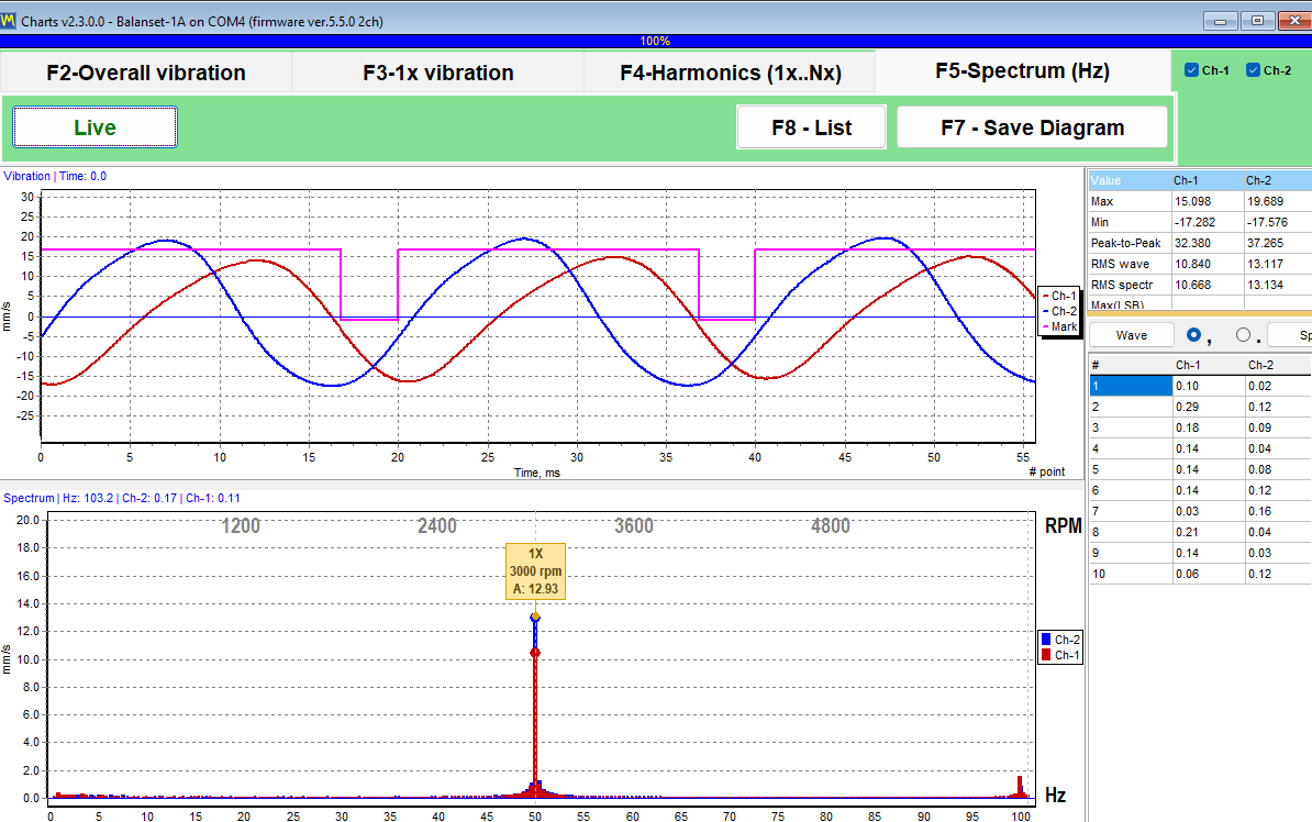
The analyser has four tabs:
- “F2 – Overall vibration” gives the broadband level per channel.
- “F3 – 1x vibration” gives the rotational component with amplitude and phase.
- “F4 – Harmonics” lists the amplitudes of the harmonics 1x to 10x as numbers.
- “F5 – Spectrum” shows the full FFT spectrum in Hz.
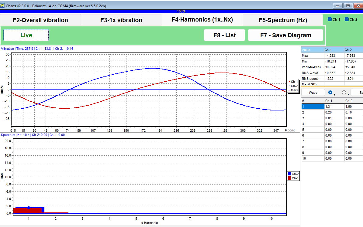
Harmonics from 1x to 10x are listed numerically, which is how an engineer separates unbalance from misalignment, mechanical looseness and blade-pass effects. Unbalance concentrates the energy at 1x, while the other faults show themselves in the higher orders. The program supplies the numbers and the interpretation stays with the engineer, which is exactly the right division of labour.
| Setting | Available values | Default |
|---|---|---|
| Frequency band | 64, 128, 320, 640 or 1024 Hz | 320 Hz |
| Accumulation length | 8, 16, 32, 64 or 128 revolutions | 16 revolutions |
| Display FFT | up to 32768 samples | — |
| Averaging | exponential, over 8 frames | — |
| RMS window | a fixed 4096-sample window, computed independently of the display FFT | — |
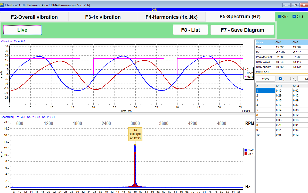
The mouse wheel zooms the chart around a peak, and the exact values are printed in the chart title rather than being left for you to estimate against the axis. For evidence and for further work, the analyser exports both pictures and raw numbers.
| File | Contents |
|---|---|
| JPEG image | The chart exactly as displayed, for a report or an email. |
| Garmoniki.txt | The harmonic table from 1x to 10x, as a plain text table. |
| WAWE.txt | The time waveform samples, as a plain text table. |
| SPK.txt | The spectrum, as a plain text table. |
All three text files open directly in Excel, so a spectrum recorded today can be compared with one recorded six months ago in whatever tool your company already uses.
One operational note that saves a support ticket: the Analyzer and the Signal Monitor stream from the same instrument over the same COM port. If both streaming windows are left open, a classic “Run 0” can fail with a port error. Close them both and repeat the run.
Bump test: finding natural frequencies (experimental)
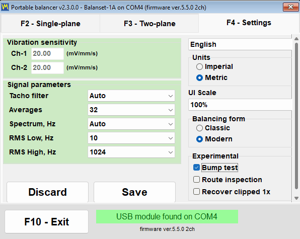
Bump test is marked experimental in the manual and is switched off by default. It is enabled with a checkbox on the “F4 – Settings” tab, after which it appears as a tab in the Vibration Meter. We describe it here exactly as the manual does, as a feature in trial use rather than a finished module.
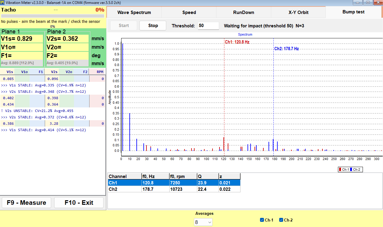
The test itself is simple. With the rotor stopped, you strike the structure next to the sensor with a soft hammer. The support rings at its own natural frequency, the program captures that ringing, and it reports per channel the natural frequency f0 in Hz and in RPM, the quality factor Q, and the damping z = 1/(2*Q). The analysis band is 12 to 600 Hz and the result is averaged over several accepted strikes.
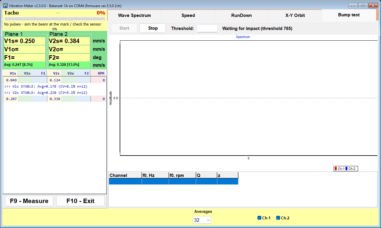
How the capture works, in numbers you can check
| Parameter | Value |
|---|---|
| Background calibration | about 0.25 s before arming |
| Trigger threshold | 8 times the measured background level |
| Capture window | about 0.6 s, including roughly a tenth of the window before the strike |
| Arming timeout | 30 s |
| Analysis band | 12 to 600 Hz |
| Clipping flag | raised at about 91 percent of the ADC scale |
The accuracy claimed by the manual, quoted without rounding it up, is about plus or minus 5 percent on Q, for Q between 20 and 100, at resonances between 80 and 400 Hz, on a clean strike. Outside that range the figure is a guide rather than a measurement.
Technique, and how to read the warnings
- Strike the structure next to the sensor, and never the sensor itself.
- Stop the rotor before striking anything.
- Avoid a double strike caused by hammer bounce, because the second impact lands inside the capture window.
- A (!) marker means the signal was clipped at roughly 91 percent of the ADC scale and the result is approximate; strike more softly and repeat.
- A steady tone message means a sustained oscillation was recorded instead of an impact, so that record is not a valid bump test.
- Only the most pronounced peak enters the result table.
The reason to use it is narrow and valuable. It tells you whether the operating speed sits near a support resonance, which is the usual reason a balancing job refuses to converge. A run-down finds the same thing while the rotor is spinning down; a bump test finds it with the machine stopped, which is sometimes the only opportunity a production schedule will give you.
How balancing works: Run 0, trial runs and the trim run
Balanset performs dynamic balancing of rotors in their own bearings. The rotor stays in the machine, on its own supports, and is balanced at its normal operating speed. Nothing is taken from a database of machines: every gram and every degree the program prints is derived from measurements made on that particular rotor during a short and fixed sequence of runs. The sequence is identical for 1, 2, 3 and 4 correction planes, and identical in both balancing forms.
Three stages, and what each one produces
| Stage | Run | What the operator does | What the program gets |
|---|---|---|---|
| 1. Initial measurement | Run 0 | Runs the rotor up to its operating speed exactly as it is, with no weights added. | The starting vibration amplitude and the phase of the 1x component in every plane. |
| 2. Trial runs | Run 1 to Run 4, one run per correction plane | Stops the rotor, fits a trial weight of known mass at a known radius and a marked angular position, runs up again, then moves the weight to the next plane. | The influence coefficients of this machine, meaning how the vibration in each plane responds to a known mass in each plane. |
| 3. Correction and check | Run T (Trim balancing) | Fits the calculated correction weights and runs the rotor once more. | Residual vibration, residual unbalance in g*mm, and a PASS or FAIL verdict against the tolerance. |
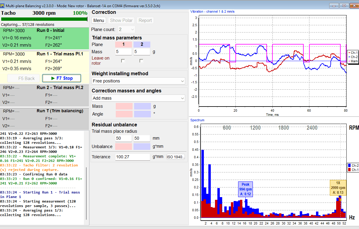
The whole measurement lives in the difference between Run 0 and each trial run. From that change the program computes the influence coefficients of the machine in front of you, and from the coefficients it computes the correction mass in grams and the installation angle in degrees for every plane at once, taking the cross-effect between planes into account.
There is no Calculate button anywhere in the program. As soon as the last trial run finishes, the calculation starts by itself and the correction mass and angle appear in the plane columns.
Sizing the trial weight
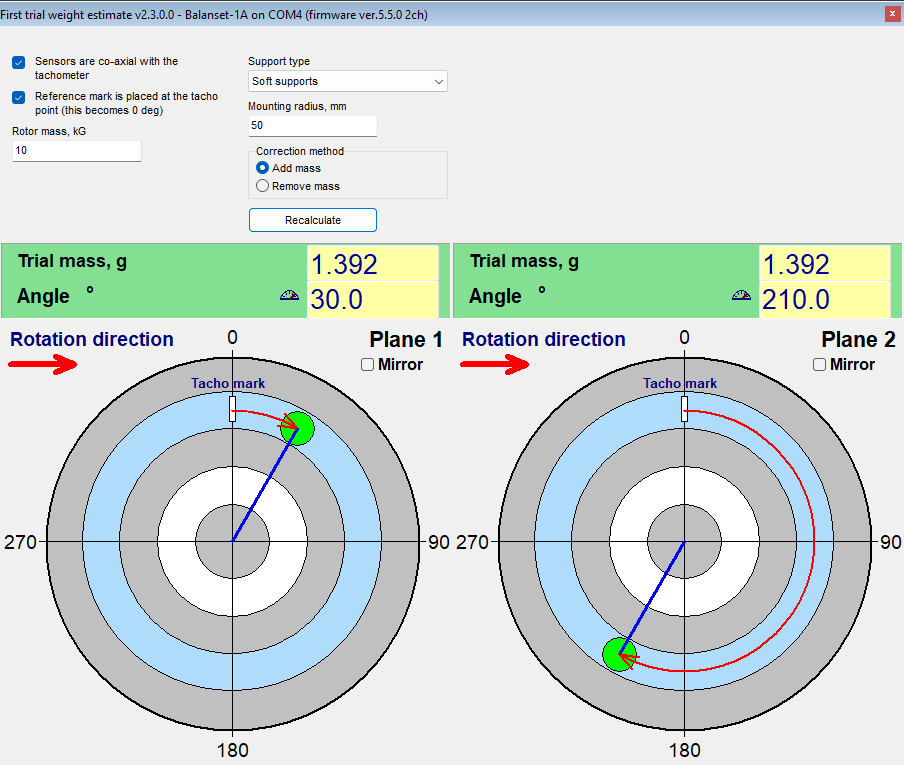
The rule of thumb is a trial weight of 0.5 to 2 percent of the rotor mass. Because that is a wide range, the program includes a “First trial weight estimate” that proposes both a mass and an installation angle from the Run 0 measurement, the rotor mass and the type of supports. It is presented here as what the manual calls it: an estimate, whose job is to put the trial weight into the correct half of the rotor rather than to be exact. It earns its keep when the trial weight has to be welded on, because moving a welded weight costs far more than measuring again.
When a trial run counts, and what to do when it does not
A trial run is only informative if the trial weight actually disturbed the rotor. The target is a change of at least 20 percent in amplitude or at least 30 degrees in phase. If the amplitude changed by less than about 10 percent and the phase by less than about 5 degrees, the run is rejected with the message “Trial weight too small. Increase trial weight and repeat Run 1”.
- Increase the trial mass by a factor of 1.5 to 2 and repeat that trial run.
- If the trial weight was installed at an angle that coincided with the phase of the original vibration, move it by 90 degrees and repeat the run.
Where the correction angle is measured from
This is the most common operator error in the whole workflow. The correction angle for a plane is measured from the point where that plane’s trial weight was installed, in the direction of rotation. It is not measured from the tacho mark. Marking the trial weight position physically on the rotor takes a few seconds and removes the ambiguity for good, including for any repeat job on the same machine.
Install the correction weight at the same radius as the trial weight of that plane. The radius is only a lever arm: it converts mass into unbalance in g*mm and does not change the correction mass in grams. The program has no way of noticing that a different radius was used, so if a different radius is unavoidable, the mass must be recalculated by hand as the calculated mass multiplied by the trial radius and divided by the actual radius.
Built-in checks against a plausible but wrong answer
Any unbalance calculation will return a number. The value of the checks below is that they stop the program from returning a confident number that the measurement does not support.
- A run whose readings did not change from the previous run is not accepted, and the program asks whether the trial weight was really installed.
- An overloaded, clipped signal is rejected instead of being processed as valid data.
- A speed that drifted between runs raises an “RPM changed significantly” warning, because influence coefficients are only valid at one speed.
- If two planes produce linearly dependent responses, the calculation is refused with “Failed to calculate influence coefficients” instead of inventing a solution. The fix is to change the mass or the angle of a trial weight and repeat the trial runs.
- Until the trial mass has been entered, the result can only be expressed as a percentage of the trial weight, and the units indicator stays on “%” instead of “g”.
One condition the program cannot check for the operator is the choice of speed. Balance at the operating speed, and not close to a support resonance, because near a resonance the amplitude is amplified and the phase drifts, so coefficients measured there do not describe the machine at its working speed.
The trim run and the BALANCING SUMMARY
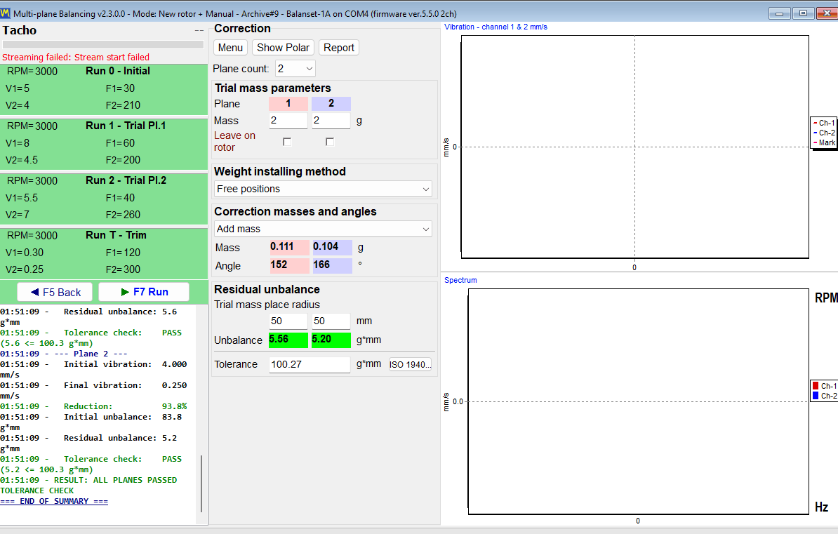
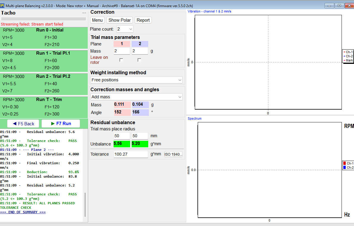
Run T verifies the correction on the real machine. After it, the program writes a “BALANCING SUMMARY” block into the log containing the vibration before and after, the reduction in percent, the initial and the residual unbalance, and a PASS or FAIL verdict for each plane. That block is the same data that goes into the HTML balancing protocol, so the number shown on screen and the number handed to the customer are the same number.
Two balancing forms: Classic and Modern (unified)
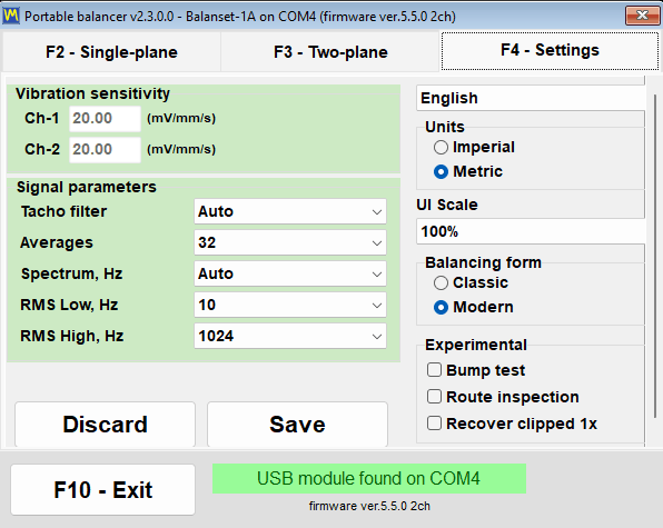
The program offers two different interfaces to the same balancing method. The switch is on the “F4 – Settings” tab, in the group “Balancing form”, and it has two values: “Classic” and “Modern”. It takes effect immediately, with no Save button to press and no restart of the program.
How many correction planes you actually get
This is the point most easily misread, so it is stated here without ambiguity. The maximum number of correction planes equals the number of vibration channels on the instrument, and 3 and 4 planes exist only in the Modern form. Balanset-1A has 2 vibration channels, so its maximum is 2 planes in either form. Balanset-4A has 4 vibration channels, so it reaches 3 and 4 planes, but only when the Modern form is selected.
| Instrument | Balancing form | Correction planes available |
|---|---|---|
| Balanset-1A, 2 vibration channels | Classic | 1 or 2 |
| Balanset-1A, 2 vibration channels | Modern | 1 or 2 |
| Balanset-4A, 4 vibration channels | Classic | 1 or 2 |
| Balanset-4A, 4 vibration channels | Modern | 1, 2, 3 or 4 |
The plane count is chosen before Run 0. Changing it rebuilds the interface and clears the measurements already taken, so it is not something to reconsider halfway through a job.
The Modern form: one window, run cards, live charts
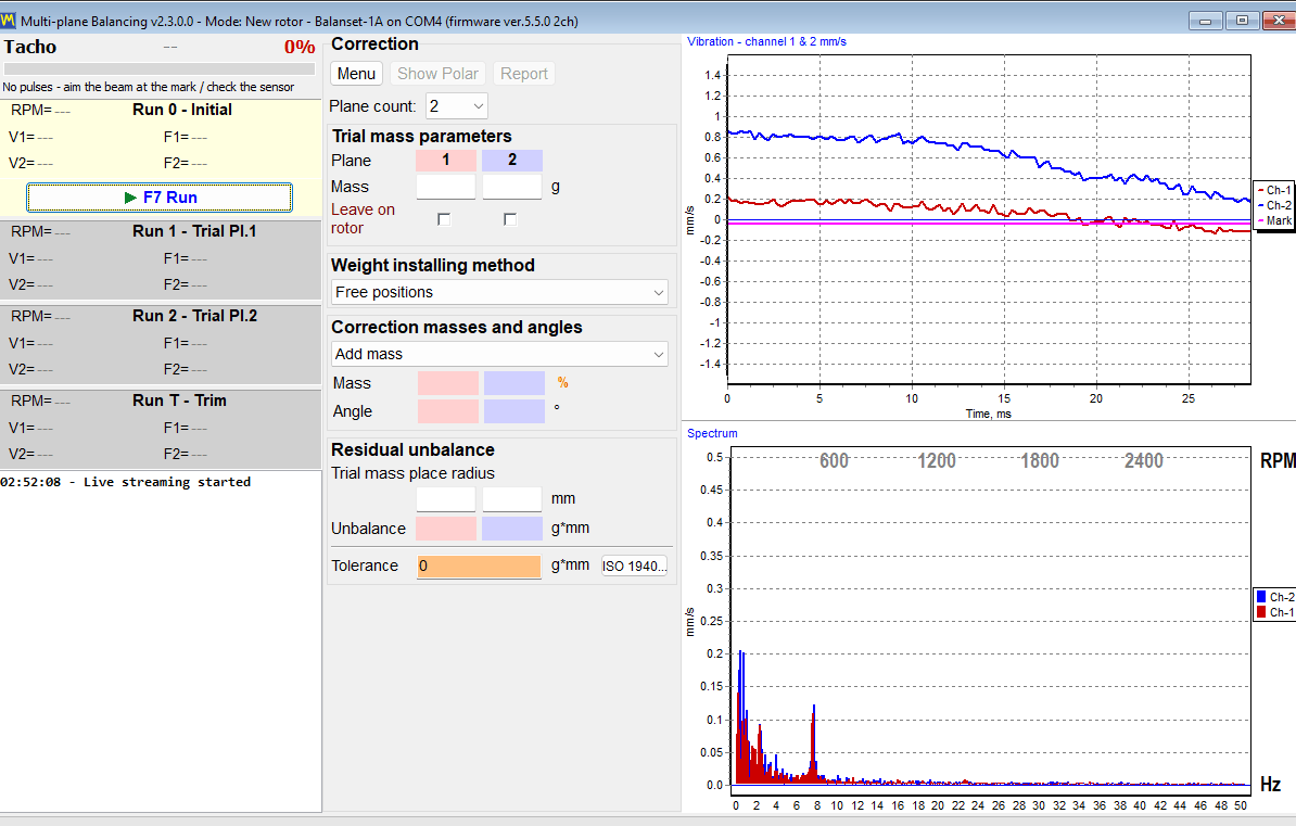
Modern is a single window called “Multi-plane Balancing”. Every run is a card in that window: “Run 0 – Initial”, “Run 1 – Trial mass Pl.1” and the equivalent card for each further plane, “Run T (Trim balancing)” and “Run E – Eccentr.”. All of them are started with the same “F7 Run” button, which becomes “F7 Stop” while a measurement is running. The waveform and the spectrum are visible during the measurement itself, so an operator can see a bad signal while it is being recorded rather than after it has been accepted.
The Classic form: two windows, one button per run
Classic keeps the layout that long-standing users already know: two separate windows, “Single-Plane balancing” and “Two plane balance”. Each run has its own button, “F7 – Run 0”, “F7 – Run 1”, “F7 – Run 2”, “F7 – Trim Run” and “F7 – Run ecc.”, and the calculated correction is read on the “Result” tab.
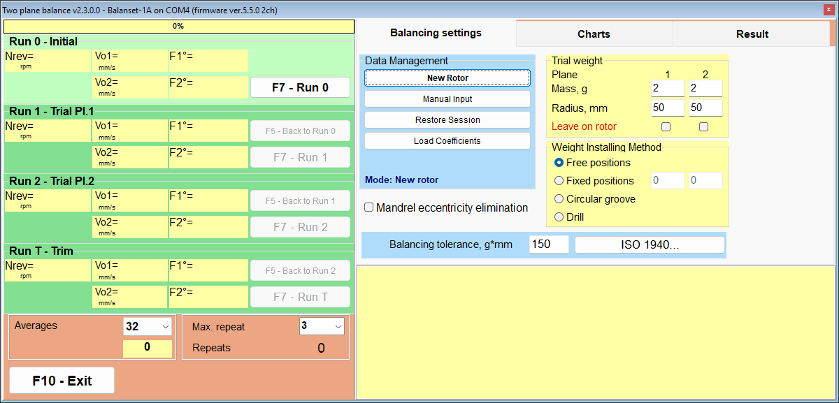
Same mathematics, different workflow
The calculation behind both forms is the same. With the same input data the result is identical, so the choice between them is a question of workflow and habit, not of accuracy.
| Aspect | Classic | Modern (unified) |
|---|---|---|
| Correction planes | 1 and 2 only | 1 to 4, with 3 and 4 on Balanset-4A |
| Windows | Two: “Single-Plane balancing” and “Two plane balance” | One: “Multi-plane Balancing” |
| Run controls | A separate button per run | Run cards driven by one “F7 Run” button |
| Calculation | Read on the “Result” tab | Starts automatically after the last trial run |
| Charts during measurement | Charts tab, switched after Run 0 | Waveform and spectrum live during the run |
| Measurement mode | “Averages” from 8 to 256, default 32, and “Max. repeat” from 1 to 20, default 3 | The same plus Auto (adaptive), or Manual (fixed repeats) with 1, 3, 5, 8, 12 or 16 repeats over 16, 32, 64, 128 or 256 revolutions |
| Loading saved coefficients | “Data Management” then “Load Coefficients” | “Menu” then “Load Coefficients” |
| Only in this form | Recalculating a finished correction into other planes with “Change corr. planes” | “First trial weight estimate”, “Manual Input”, adaptive measurement, 3 and 4 planes |
In Auto (adaptive) mode the program extends the measurement until the result settles and shows a convergence indicator while it does so. If it reports “Additional averaging does not improve accuracy”, that is a statement about the machine and not about the software: the usual causes are loose mountings, worn bearings or an unstable speed, and more averaging cannot repair any of them.
The recalculation function unique to Classic deserves one operating note. “Change corr. planes” has to be clicked with the mouse, because in that window the F5 key acts as Back rather than as the labelled command.
The two forms share one archive. Records made with 3 or 4 planes always open in the Modern form, because Classic has no interface able to display them.
Where to put the weight: correction methods and polar diagrams
A calculated mass and angle is only half an answer. The other half is whether that position can be reached on the real rotor, which is why the program carries four weight installation methods, selected per plane in “Weight installing method”, and recalculates the correction into the form each one needs.
| Method | What the program outputs | Condition or limit |
|---|---|---|
| Free positions | One weight, at exactly the calculated angle. | For rotors where any angular position can be reached. |
| Fixed positions | The correction split between two adjacent numbered positions, such as fan blades or existing holes. | At least 3 positions are required. Above 32 positions the polar diagram is not drawn. |
| Circular groove | Three equal weights spaced about 120 degrees apart. | Refused with “TOO HEAVY for 3-weight groove method!” if the correction exceeds one third of that plane’s trial mass. |
| Drill | Drilling depth H, number of holes N and angle f. | Always switches the method to Remove mass. |
Polar diagrams: the check before anything is fitted
The polar diagram is the operator’s last look before touching the machine. Up to 4 circles are shown side by side, one per correction plane, with rings at 20, 40, 60, 80 and 100 percent and an arrow showing the direction of rotation. Seeing the weight drawn on a circle that turns the same way as the rotor is what catches an angle counted the wrong way round, which is the failure mode that costs an extra run.
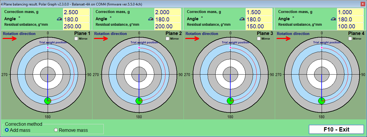
Two switches change how the same solution is expressed. “Add” and “Remove” converts an add-mass solution into a remove-mass solution by rotating the angle 180 degrees at the same mass, which is what you want when the practical option is grinding or drilling rather than welding. “Mirror” flips the angular display for a plane, showing for example 60 degrees in the place of 300 degrees, for rotors that are physically accessed from the other side.
Fixed positions: fan blades and existing holes
On a fan, an impeller or a flange with a bolt circle, a weight can only go where there is somewhere to put it. In “Fixed positions” the operator enters how many positions the rotor has, numbered in the direction of rotation, and the program splits the correction between the two adjacent positions that bracket the calculated angle, giving a mass for each. The result is directly executable: two numbers, two blades.
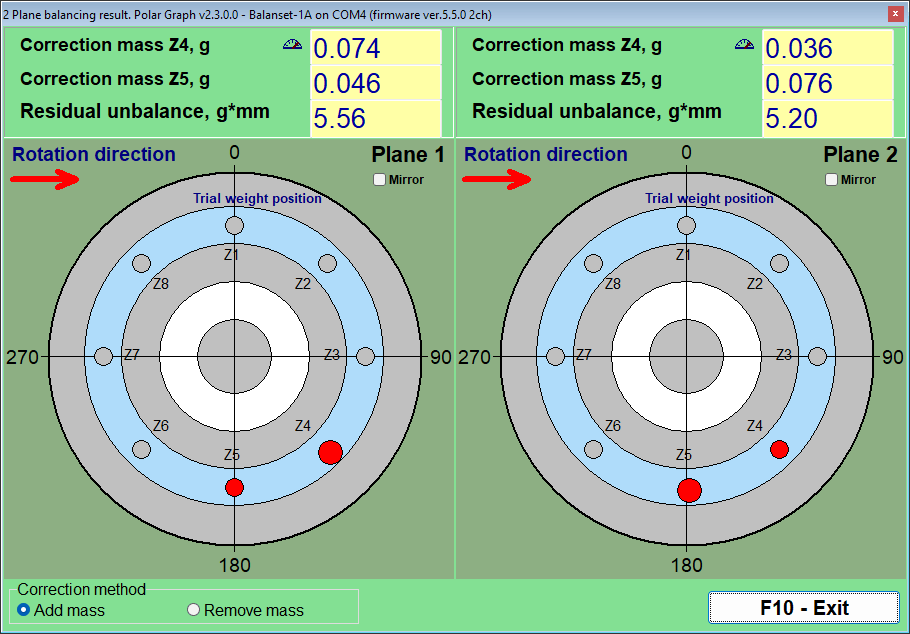
Circular groove: three weights at about 120 degrees
Rotors with a circular groove, such as many grinding wheel arbors, take standard weights that slide in the groove. Here the correction is expressed as three equal weights spaced about 120 degrees apart, whose vector sum equals the required correction. The method has a physical limit built in: if the correction is larger than one third of that plane’s trial mass, the program refuses it with “TOO HEAVY for 3-weight groove method!” instead of proposing weights that would not fit the scheme.
Drill: turning a correction into holes
When mass has to be removed rather than added, the built-in calculator in the “Drilling – settings” window converts the correction into the drilling depth H, the number of holes N and the angle f. It needs three inputs: the drill diameter, the maximum allowed drilling depth and the material density. Choosing Drill always switches the method to Remove mass.
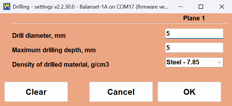
Densities are preset in g/cm3 for Steel 7.85, Cast iron 7.1, Aluminum 2.7, Copper 8.95, Brass 8.5, Bronze 8.8 and Titanium 4.5, and a custom value can be typed in for any other material.
Two honest notes about the drilling calculator. Because the conical tip of the drill is accounted for, the displayed H can come out slightly larger than the maximum depth that was entered, so it must always be checked against what the part mechanically tolerates. If the depth would be exceeded, the correction is divided across several adjacent holes, and that result should be confirmed with a trim run rather than assumed.
Mandrel eccentricity: the Run E compensation
A rotor balanced on a mandrel carries an error that has nothing to do with unbalance: the runout of the mandrel itself. The program handles it with a dedicated eccentricity run, “Run E – Eccentr.” in the Modern form and “F7 – Run ecc.” in Classic. The rotor is turned 180 degrees on the mandrel and measured again, which separates the runout component from the true unbalance so that only the unbalance is corrected.
When the calculated plane cannot be reached
Sometimes the correct correction plane is simply not accessible with a tool. The Classic form can recalculate a finished two-plane correction from the planes it was computed for, H1 and H2, into two other planes, K1 and K2, using the rotor geometry. Four geometry schemes cover the usual arrangements of the new planes relative to the old ones, and the distances between them are entered in mm together with the new radii. The result is the same unbalance expressed as weights you can actually fit.
Tolerances and standards: ISO 1940 and ISO 10816-1
A balancing job is only finished when somebody can say, on paper, that the rotor is inside a documented tolerance. The Balanset software applies two different standards to two different questions. ISO 1940 answers the acceptance question at the end of a balancing job: is the residual unbalance small enough for this type of rotor? ISO 10816-1 answers the condition question during monitoring: is this machine running in zone A, B, C or D? Both criteria are built into the program, and every number used by them is printed below so you can check the arithmetic against your own machine before you buy anything.
ISO 1940: the residual unbalance is checked automatically, plane by plane
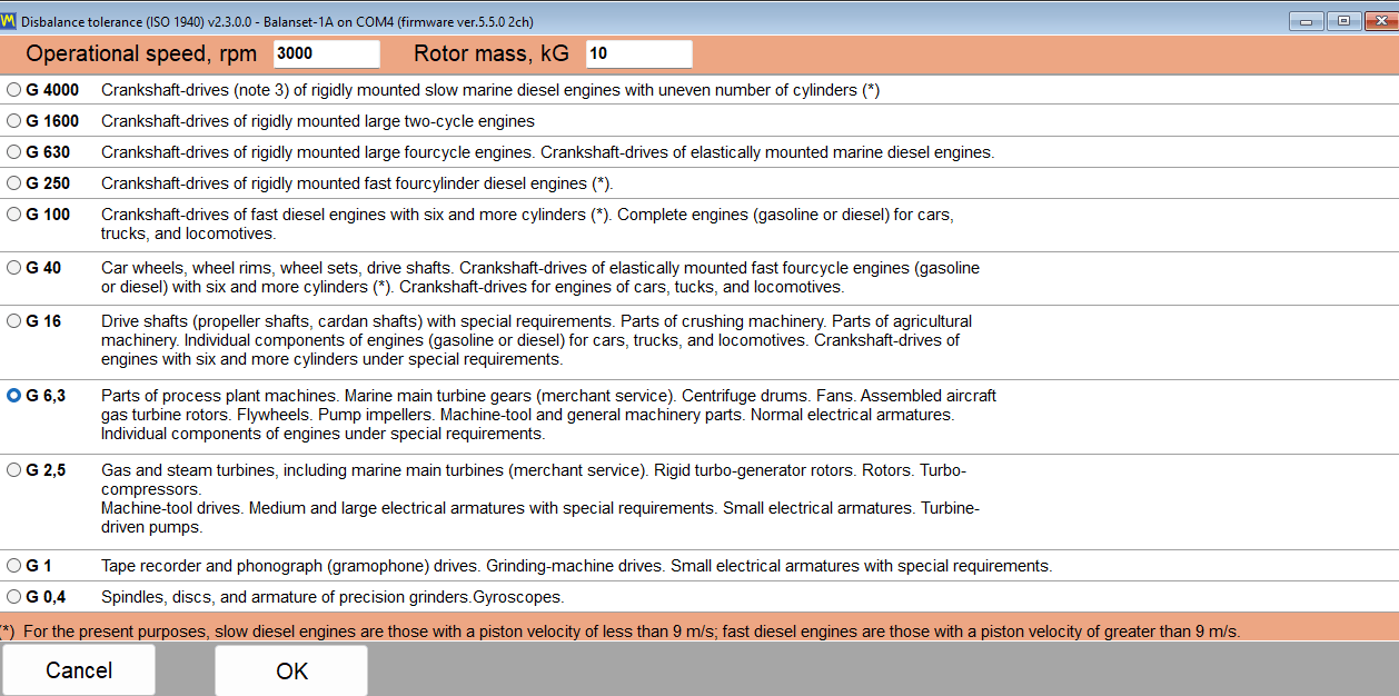
The tolerance is set once, before Run 0, with the “ISO 1940…” button, which opens the “Disbalance tolerance (ISO 1940)” window. You enter the balance quality grade G, the rotor mass and the operating speed, and the program stores the resulting permissible residual unbalance together with the session. After the trim run the measured residual unbalance is compared against that value: the field is highlighted green when the result is inside the tolerance and red when it is not, and the program states an explicit PASS or FAIL for each correction plane. Nothing has to be looked up in a table by hand, and nothing depends on the operator’s judgement of what “good enough” means.
The formula, printed in full so it can be verified
The program uses the standard ISO 1940 expression, and there is nothing hidden behind it:
Uperm [g*mm] = 1000 * G * M / (2 * pi * f)
Here G is the balance quality grade in mm/s, M is the rotor mass in kg, and f is the operating speed in Hz, that is RPM divided by 60. The worked example from the manual is easy to repeat on a calculator: grade G 6.3, a speed of 3000 RPM and a rotor mass of 10 kg give a permissible residual unbalance of about 200.5 g*mm. When two correction planes are used, the permissible unbalance is split equally between them, so each plane is judged against Uperm / 2 rather than against the whole figure.
Because the tolerance is derived from your own three inputs, the verdict on the screen is reproducible by anyone who reads the report, including your customer’s inspector.
Choosing the balance quality grade
The “Disbalance tolerance (ISO 1940)” window offers the grades G 4000, G 630 to G 100, G 40, G 16, G 6.3, G 2.5, G 1 and G 0.4. The table below repeats the application hints shown in that window, so the grade can be chosen before the instrument is even connected.
| Grade | Typical application |
|---|---|
| G 4000 | Crankshafts of very large, slow-running marine diesel engines |
| G 630 to G 100 | Crankshafts of large and high-speed diesel engines, and complete engines |
| G 40 | Car wheels, rims and drive shafts |
| G 16 | Propeller and drive shafts, parts of crushers and agricultural machines |
| G 6.3 | Fans, pump impellers and machine tool parts; the usual general industrial default |
| G 2.5 | Gas and steam turbines, rigid turbogenerator rotors |
| G 1 | Grinding machine drives and small armatures |
| G 0.4 | Precision spindles, discs and gyroscopes |
For most field work on fans, blowers, pump impellers and machine tool components, G 6.3 is the grade that will be expected of you, and it is the one to start from unless the machine builder specifies otherwise.
ISO 10816-1: machine classes and vibration zones
Assessing the condition of a machine is a separate question from accepting a balancing job, and the program uses a separate standard for it. Overall vibration velocity is scored against ISO 10816-1 machine classes I to IV, the classification formerly published as ISO 2372, with the four zones A, B, C and D. Zone A is a newly commissioned machine, zone B is acceptable for unrestricted long-term operation, zone C means the condition is only acceptable for limited operation, and zone D means the vibration is severe enough to cause damage. The thresholds are published here in full, in mm/s.
| Class | Machines | A/B, mm/s | B/C, mm/s | C/D, mm/s |
|---|---|---|---|---|
| Class I | Small machines | 0.71 | 1.8 | 4.5 |
| Class II | Medium machines | 1.12 | 2.8 | 7.1 |
| Class III | Large machines on a rigid foundation | 1.8 | 4.5 | 11.2 |
| Class IV | Large machines on a compliant foundation | 2.8 | 7.1 | 18.0 |
One point of honesty is worth stating clearly, because vibration standards are easy to blur in marketing text. The program uses the machine class table of ISO 10816-1, classes I to IV. It does not use the group and support type scheme of ISO 10816-3. If your acceptance procedure is written against ISO 10816-3, the class thresholds above are a practical screening criterion, not a substitute for that document.
The measurement band behind the number
A vibration severity figure only means something if the frequency band it was measured in is known. The default upper limit in the program is RMS High, Hz = 1024, which matches the usual 1 kHz convention behind the ISO 10816 tables. The default lower limit is RMS Low, Hz = 10. For machines running below 600 RPM, ISO 10816-3 asks for a broadband RMS starting at 2 Hz, so on such machines the lower limit should be reduced to 1 or 2 Hz before the reading is compared with any zone table. This is a setting the operator controls, and it changes the number on the screen, which is exactly why it is documented here rather than buried.
Past jobs stay auditable
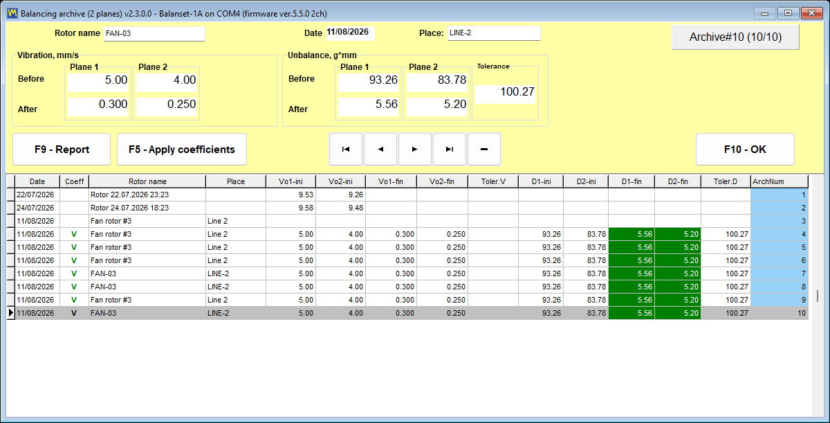
The tolerance verdict is not only a live indication. Records in the session archive are coloured according to their residual unbalance against the stored tolerance, so a whole list of previous jobs can be scanned at a glance for results that fell outside the limit. For a service company this is the difference between having done the work and being able to prove it a year later.

Session archive, repeat balancing without trial runs, and reports
Trial runs are the expensive part of a balancing job. Every one of them means stopping the rotor, fitting a weight, starting up again and waiting for a steady speed. The session archive exists so that this work is paid for once per machine instead of once per visit, and so that the paperwork handed to the customer is produced by the program rather than typed up afterwards.
Every session is archived, with the coefficients that made it work
An archive record is written automatically; there is no dialog to remember at the start of the job. Together with the measurements the program stores the influence coefficients it calculated for that machine, the trial masses, the trial mass radii, the number of fixed positions and the tolerance that was in force. When the balancing window is closed, the program asks for the rotor name and the place of installation, so the record can be found again by a human rather than by a number.
Balancing the same rotor again does not require new trial runs
This is the part that a service company actually pays for, and it is worth stating as a mechanism rather than as a slogan. The influence coefficients describe how that particular machine responds to a weight in each plane. Once they are stored, a repeat job on the same rotor only needs the initial measurement: the saved coefficients are loaded, Run 0 is measured, and the correction masses and angles are calculated immediately. The trial runs are not repeated at all.
There are three ways to load stored coefficients:
- In the Modern form, “Menu” and then “Load Coefficients”.
- In the Classic form, “Data Management” and then “Load Coefficients”.
- From the main window, F8, then select a record that shows a green V in the “Coeff” column and press “F5 – Apply coefficients”.
Two caveats have to be published with that promise, because ignoring either of them produces a confident but wrong result.
- In the archive, “F10 – OK” does not load a session and does not transfer any coefficients. Only “F5 – Apply coefficients” does that. This is the single most common misunderstanding of the archive window.
- Coefficients are valid only for the same machine and the same rotor type, with unchanged sensor positions and an unchanged running mode. For that reason the trial weight location should be marked physically on the rotor during the first job, so the next visit starts from the same geometry.
The result of a repeat job is saved as a new archive record. The original record is not modified, so the history of the machine stays intact.
Trim iterations cost almost nothing
If the residual unbalance is still above the tolerance after the trim run, the trial runs are not repeated either. The coefficients already exist, so the program calculates the additional correction straight away. The extra weight is added without removing the weights that are already fitted, and the trim run is repeated. This can be done as many times as the job needs, which is why a difficult rotor costs time in start-ups rather than in measurement work.
Reports the program writes for you
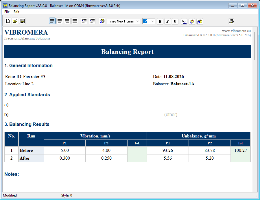
Three HTML documents are produced by the software itself, all encoded in UTF-8 and all openable in any browser on any operating system, including a customer’s phone:
protocol11.htm, the balancing protocol for a completed job.vibrometer_report.htm, the vibration meter report for a measurement session.report_YYYY-MM-DD.htm, the route report for one inspection day.
A report is not a dead end file. The program includes a report editor with a print preview, and the preview can be zoomed from 10 to 200 percent from the list, or up to 500 percent by entering the value manually, which matters when checking a small number on a laptop screen next to a machine.
Export formats, and the one requirement nobody expects
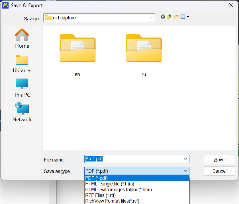
| Format | Typical use |
|---|---|
| The document sent to a customer or attached to a work order | |
| HTML, single file | One self-contained file with the images embedded, easy to e-mail |
| HTML with an image folder | Editable version for publishing or for pasting into another document |
| RTF | Opening and editing the protocol in a word processor |
| RVF | Native rich text format of the built-in editor |
One requirement has to be stated plainly, because it surprises people on a fresh laptop: PDF export needs at least one Windows printer to be installed. The printer driver is used only to compute the page layout, and nothing is actually printed. If the computer has no printer at all, enable “Microsoft Print to PDF” in Windows and the export will work.
Your letterhead, your logo
Report templates are ordinary HTML files in the bin\ReportTpl\ folder and can be edited so that the protocol carries your company letterhead, logo and contact details. Edits are preserved across automatic updates, stored as name.user-*.htm files, but they are not merged into a new template automatically, so after an update that changes a template the customisation has to be carried over by hand. That is a limitation, not a feature, and it is better known before the first update than after it.
The data is yours and it is portable
The archive and the reports live in Documents\BalSoft\Bs1A. They survive program updates and a full reinstallation, and they move to another computer by copying that folder. There is no database server to migrate, no licence server to contact and no cloud account holding your measurement history.
Route Inspection: walk-around monitoring by ISO 10816-1 (experimental)
Route Inspection is marked as experimental in the user manual and it is disabled by default. It is switched on with a checkbox on the “F4 – Settings” tab. We state that first, before describing what it does, because the module is genuinely useful but it is not presented by the manufacturer as a mature condition-monitoring platform, and you should not buy the instrument on the strength of this module alone.
What it adds is a second life for the same hardware. Between balancing jobs, the instrument and the laptop become a walk-around vibration monitoring set: you follow a defined route through the plant, measure the same points in the same way every time, and watch the numbers move.
How a route is organised
The data model has three levels, and it maps onto the way a plant is actually walked:
- A route is one walk-around, for example a workshop or a production line.
- A point is a machine on that route.
- A spot is one bearing combined with one axis, which is what the sensor actually measures.
A point can hold up to 8 bearings, and each bearing has 3 axes: X horizontal, Y vertical and Z axial. That gives a maximum of 24 measurement spots on a single machine, which is enough for a multi-stage pump or a motor and fan set with several supports.
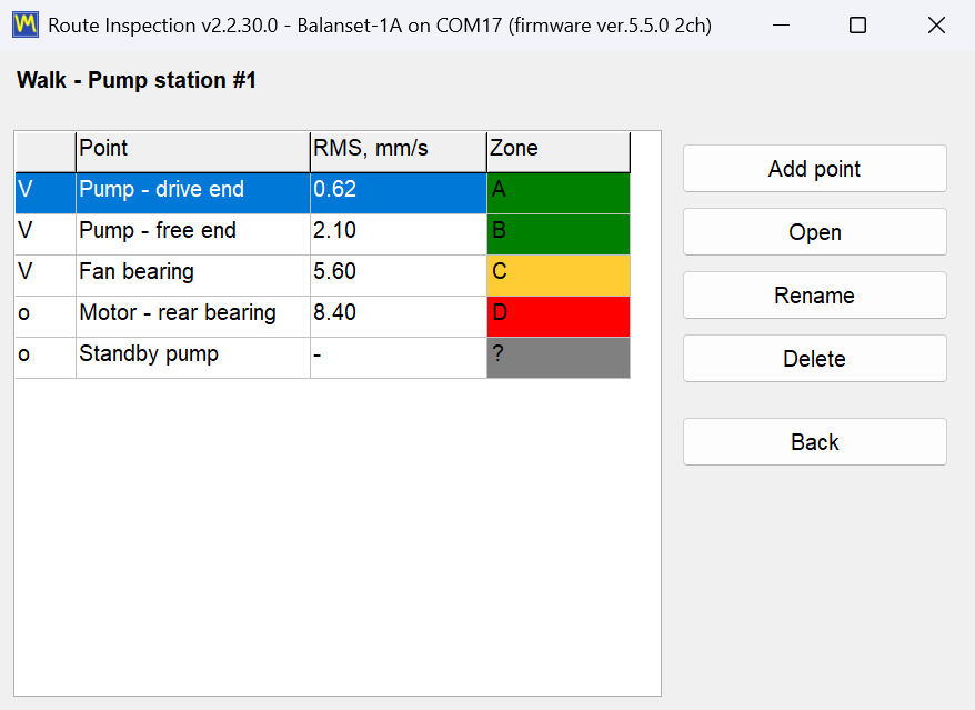
Every spot is scored against ISO 10816-1
Each measured spot is compared with the ISO 10816-1 thresholds for the machine class you assigned to that point, classes I to IV, and is coloured by zone A, B, C or D. That colour is the point of the module during a walk: an unmeasured point is visually distinct from a healthy one, so it is obvious at the end of the round whether the route was completed, and obvious immediately which machine needs attention before you have opened a single chart.
Trends and the forecast
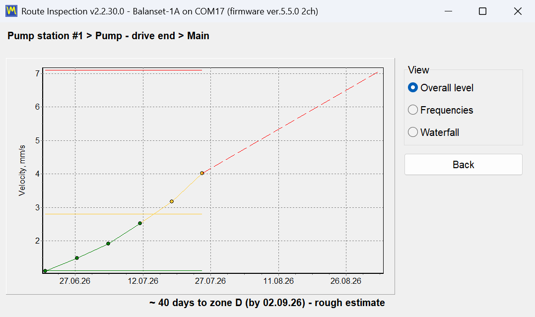
Three trend views are available for each spot. “Overall level” plots the broadband vibration velocity over successive visits against the ISO 10816-1 zone boundaries. “Frequencies” follows individual frequency components, which is how a developing bearing fault separates itself from a slow rise in unbalance. The waterfall view stacks up to the 12 most recent channel 1 spectra, so a new peak that was not there three visits ago becomes visible as a ridge rather than as a number.
The program also extrapolates. Using up to the 6 most recent visits it fits a straight line and phrases the outcome as approximately N days to zone X. It is important to present that exactly as the manual does: it is a rough estimate for maintenance planning, produced by linear extrapolation of a handful of points. It is not a guaranteed remaining life, and a fault that develops non-linearly will not respect it. Used honestly, it is a way of deciding which of two machines to schedule first.
What a visit can carry besides numbers
A vibration reading on its own often loses the context that made it meaningful. Each visit can therefore also record a free text note, a temperature reading and a photo in jpg, png or bmp format, so that the loose guard, the oil leak or the temporary coupling is documented next to the measurement that it explains. A run-down of up to 120 s can also be recorded inside the route, which means a coast-down of a suspicious machine can be captured during the walk instead of being scheduled as a separate visit.
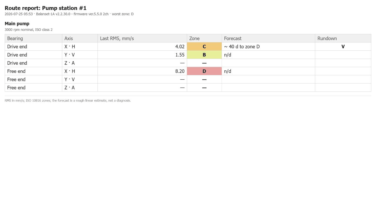
The route report
One HTML report is produced per inspection day, named report_YYYY-MM-DD.htm. It is the document that goes to the maintenance planner or to the customer at the end of the round, and like the other reports it opens in any browser without the software being installed on the reader’s computer.
Operational notes worth knowing in advance
- If no COM port has been accepted, the measurement buttons are not greyed out. They answer “Measurement is not available.” instead, so a missing instrument looks like a refusal rather than like a disabled interface.
- Opening a route window stops a running Signal Monitor or Run-down. The instrument has a single port, and the route module takes it over. This is expected behaviour, not a fault.
- Reducing the number of bearings on a point is blocked if the bearing that would disappear already has measurement history. The program protects the trend rather than the layout.
- Deleting a route or a point does not erase the data. The folder is moved to
Routes\_deleted, so a deletion made in the field can be undone back at the office.
The data stays readable outside the program
Route data is stored in plain files, in SI units, with a decimal point regardless of the Windows regional settings. That last detail sounds trivial and is not: it means a route recorded on a laptop configured for a language that uses a decimal comma opens correctly on any other machine, and the files can be parsed by your own tools without a converter.
Settings, units, languages and screen scaling
Everything that changes how the program measures and how it looks sits on one tab of the main window, “F4 – Settings”. There is no nested tree of preference dialogs to hunt through: sensor sensitivity, the signal parameters, the interface language, “UI Scale”, the “Units” system, the “Balancing form” switch and the “Experimental” feature checkboxes are all on the same screen, and the values you see there are the values the instrument is using right now.
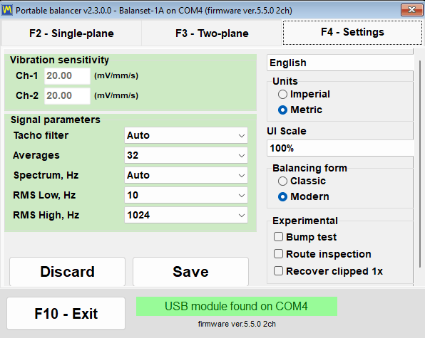
Two buttons at the bottom left control persistence. “Save” writes the current settings into the Bs1A.cfg configuration file so that they become the defaults at the next start, and “Discard” cancels unsaved changes and re-reads the values from that file. Most parameters — “Tacho filter”, “Averages”, “Spectrum, Hz”, the RMS band and the unit system — take effect the moment you change them, and they are written to Bs1A.cfg automatically when the program exits normally. Language, “UI Scale”, “Balancing form” and the experimental checkboxes are written to the file immediately on change, so for those you never need to press “Save”.
Sensor sensitivity, locked on purpose
The “Vibration sensitivity” group holds one coefficient per channel in mV/(mm/s), and the factory value for the supplied accelerometers is 20. The Ch-3 and Ch-4 fields exist only on a four-channel Balanset-4A. The fields are protected against accidental edits: nothing can be typed into them until you click the group and confirm the “Do you really want to change it?” prompt. That single question is what stops an operator from silently recalibrating the whole instrument with a stray keystroke in the middle of a field job. Change these numbers only if your sensor differs from the standard one.
Signal parameters
| Parameter | Values | Default | What it changes |
|---|---|---|---|
| “Tacho filter” | “Auto”, “Fine (1%)”, “Normal (2%)”, “Coarse (5%)”, “Very coarse (10%)”, “Rough (20%)”, “Off (40%)” | “Auto” | The permissible speed variation between adjacent revolutions |
| “Averages” | 8 / 16 / 32 / 64 / 128 / 256 | 32 | The number of averaged FFT spectra: more gives a smoother spectrum and less noise, but a slower update |
| “Spectrum, Hz” | 100 to 8000, or “Auto” | “Auto” | The maximum frequency shown on the spectrum; “Auto” picks the range from the rotation speed |
| “RMS Low, Hz” | 1 to 10 | 10 | The lower bound of the overall vibration level band |
| “RMS High, Hz” | 1024 / 2048 / 4096 / 8192 | 1024 | The upper bound of the RMS band; 1024 corresponds to the ISO 10816 convention of 1 kHz, larger values are for high-speed machinery |
The “Auto” tacho filter picks its tolerance adaptively: it starts at 2 percent and, if the rotation is uneven, relaxes in steps up to 40 percent while flagging the measurement as taken at reduced accuracy. For the live stream in the Vibration Meter, “Auto” corresponds to a fixed 20 percent. The trade-off is worth knowing before you touch it: too strict a filter throws the rotation speed away entirely on a belt drive or a vibrating support, and too loose a filter accepts the measurement but reduces phase accuracy.
Metric and Imperial units
The unit system is switched in the “Units” group, between “Metric” (the default) and “Imperial”. The switch covers every quantity the program handles, on screen and in the reports alike.
| Quantity | Metric | Imperial |
|---|---|---|
| Weight mass | g | oz |
| Radius and length | mm | in |
| Unbalance (moment) | g*mm | oz*in |
| Vibration velocity | mm/s | inch/s |
| Rotor mass for ISO 1940 | kg | lb |
| Material density | g/cm3 | oz/in3 |

Internally the program always computes and stores data in SI, that is in g, mm, g*mm, mm/s and kg, and converts only on input and on display. This is the reason an archive record or a saved session does not break when a colleague opens it with the other unit system selected. After switching, the unit labels on every window, chart and report update immediately, but numbers that were already entered and already shown are not recalculated automatically, and the program says so and recommends a restart for full consistency. Small correction masses are displayed with adaptive precision down to 0.001 g, or 0.001 oz, so the value of a fine weight is not lost to rounding.
27 interface languages
The program and its manual are translated into 27 languages: English, Bulgarian, Czech, Danish, German, Estonian, Spanish, French, Indonesian, Italian, Latvian, Lithuanian, Hungarian, Dutch, Norwegian, Polish, Portuguese, Portuguese (Brazil), Romanian, Russian, Slovak, Slovenian, Finnish, Swedish, Turkish, Ukrainian and Japanese. The language list is in the top-right corner of the settings tab.
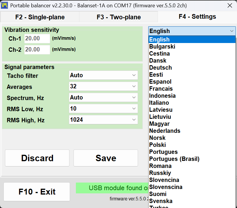
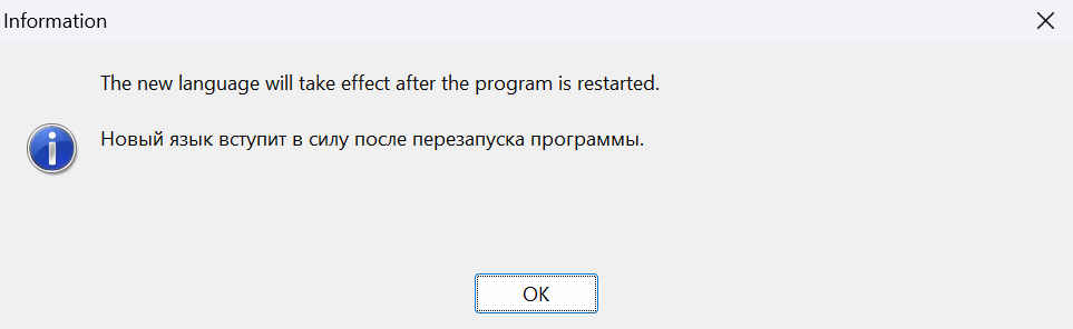
The names in the list are written in the Latin alphabet, so Russian appears as “Russkiy” and Japanese is offered in Romaji, which means you can always find your way back even after switching to a language you cannot read. The choice is written to Bs1A.cfg at once and applies after the program is restarted; the notice “The new language will take effect after the program is restarted.” is deliberately shown in two languages at the same time, the current one and the one you have just selected. The interface language also controls the labels inside the HTML reports, so a balancing protocol handed to a customer comes out in the customer’s language.
UI Scale for field laptops
“UI Scale” offers 100, 125, 150, 175 and 200 percent, and it is applied on top of the Windows system DPI scale, so the final size of the elements is the combination of the two. Like the language, the scale takes effect after the program is restarted. In the “Vibration Meter” and “Charts” windows the Maximize button additionally scales fonts, buttons, fields and chart axes to the available screen area, and restoring the window returns the base scale; this behaviour is on by default and can be turned off only in the configuration file with the key MaximizeZoom=0 in the [UI] section. Every window is kept inside the desktop work area, so at 150 and 200 percent a dialog no longer runs behind the taskbar or clips its bottom row of buttons, and the program shrinks the font of a label or a button automatically when a long translation does not fit.
Balancing form and the experimental switches
The “Balancing form” group decides which window the “F6 – Balancing” button opens, “Classic” or “Modern”. The choice is saved immediately and applies the next time the balancing window is opened, with no restart. The group itself appears only after the program has identified a connected device with supported firmware; until then it stays hidden, while the value previously saved to Bs1A.cfg remains in force.
The “Experimental” group carries three checkboxes, all of them off by default. “Bump test” adds the natural-frequency tab to the Vibration Meter. “Route inspection” adds the “F9 – Route Inspection” button, and toggling it rebuilds the main window right away without a restart. “Recover clipped 1x” changes what happens when the vibration signal goes off scale: instead of rejecting the measurement, the program reconstructs the rotational component from the undistorted portions of the signal, at reduced accuracy, and marks the result as approximately reconstructed. The “Bump test” checkbox, like the “Balancing form” group, becomes effective only once a device with supported firmware has been identified.
Bs1A.cfg: the settings are a plain text file
All settings are stored in a single text INI file, Bs1A.cfg, which lives next to Bs1A.exe. The program does not use the Windows registry at all. The file can be edited by hand while the program is closed, which is the simplest way to roll out an identical configuration across a fleet of service laptops: copy one file. Numeric values for sensitivity, noise floor, presets and drilling are accepted with either a decimal point or a decimal comma, so changing the interface language or the Windows regional format does not reset them.
Installation, system requirements and where your data is kept
The Balanset software is an ordinary Windows desktop application. You install it once on the laptop that will go to the machine, and from then on the instrument is just a USB device that the program finds by itself.
| Parameter | Requirement |
|---|---|
| Operating system | Windows 7, 8, 10 or 11, 32-bit or 64-bit |
| Port | One free USB port |
| Disk space | About 150 MB |
| Display | 1024×768 or higher; 1366×768 and above recommended |
| Administrator rights | Not required |
| Internet connection | Not required for measuring, balancing or reporting |
Two ways to install
The wizard install is the recommended route on a computer that has never had the program. Run Bs1ASetup.exe and step through the wizard; the default location is the current user’s Documents\BalSoft folder, and the program lands in the Bs1A subfolder, giving Documents\BalSoft\Bs1A\Bs1A.exe. The instrument does not have to be connected while you install. One instruction in that wizard is worth reading twice: do not clear the “Encoder driver setup” or the “DB setup” options, because without the database component the session archive will not work. At the end the wizard creates a “Bs1A” desktop shortcut and a Start menu group containing the program, the manual and a link to the manufacturer’s site.
The program is also portable. It does not touch the Windows registry, and all of its settings live in Bs1A.cfg next to the executable, so the whole application can be unpacked into any convenient folder and run from there — including from a USB stick that travels with the instrument. Two caveats apply. Do not unpack it into Program Files, because writing settings there needs administrator rights. And if the computer has never had the wizard install, the portable copy has neither the database component nor the instrument driver, so run the wizard once on that machine; after that you can update by any method.
First run
Start Bs1A.exe and the main window opens with the program version in the title bar. The connection status line at the bottom of the window tells you immediately which of three situations you are in: “USB module found on” with the COM port number means the instrument is ready, “USB module not connected” means it was not found, and “Firmware not supported on COM…” in red means the instrument answered but its firmware is older than 5.5.0. The program never opens twice — starting it again simply brings the existing window to the front and restores it if it was minimized — because two instances would compete for the same COM port.
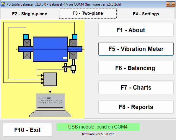

You can install and explore the program before the hardware ever arrives. With no instrument attached the main window still opens and stays fully usable — there are no blocking dialogs — and the status line simply reports that nothing was found. Choosing your language is usually the first thing to do after installation: pick it on the “F4 – Settings” tab, then close the program with “F10 – Exit” and start it again.
Where the files are
| What | Where | Note |
|---|---|---|
| Settings | Bs1A.cfg, next to Bs1A.exe | Plain INI text; language and scale are written the moment they change |
| Session archive and reports | Documents\BalSoft\Bs1A | Always in the current user’s Documents folder, wherever the program itself is installed |
| Operation logs | The logs folder next to Bs1A.exe | bs1a.log plus bs1a.1.log to bs1a.5.log, capped at 5 MB per file and 5 files |
| Report templates | The ReportTpl folder next to Bs1A.exe | Editable, so the protocol can carry your own letterhead |
| Window screenshots | Documents\Bs1A\Screenshots | Written by the F12 key as PNG files |
Because the archive is deliberately kept in the user’s Documents folder rather than beside the executable, it survives program updates and even a full reinstall, and on the first run of a new version the program copies an archive found in the old location into Documents\BalSoft\Bs1A without deleting the original. Moving a technician to a different laptop therefore means copying two folders: the program folder, which carries Bs1A.cfg and your report templates, and Documents\BalSoft\Bs1A, which carries every balancing session you have ever recorded. There is nothing to deactivate, transfer or re-license.
Connecting the instrument, and the firmware 5.5.0 requirement
Connect the vibration sensors to the channel connectors Ch-1 to Ch-4 marked on the case — two of them on a Balanset-1A, four on a Balanset-4A — and the laser tacho to the Tacho connector. On older revisions of the case the same inputs are marked X1 and X2 for vibration and X3 for the tachometer, so do not be surprised if the labels on your unit differ. Mount the vibration sensors on the bearing supports of the rotor being balanced, stick a reflective mark on the rotor, and connect the USB module to the computer with the USB cable. The order is not strict, because the device is picked up at any moment, including while the program is already running.
One detail causes more support calls than any other: the tachometer is powered through its own cable from the instrument and needs no batteries, so there is no reason to open the battery-compartment cover. After connecting it, press ON and then AUTO on the sensor, and the laser beam should light up.
There is no Connect button
The program scans the COM ports by itself, roughly every 1.5 seconds, finds the device and queries its firmware. The port that was found is remembered, so the next start connects faster. A port held open by another program does not stop the scan — the remaining ports are still checked, and the busy one is tried again on a later cycle — and a foreign Arduino board on a neighbouring port does not block the search either. On Windows 10 and Windows 11 the COM port driver installs automatically; in Device Manager the instrument appears as a COM port named “Arduino Due”. Clicking the USB status line forces an immediate search instead of waiting for the next cycle.
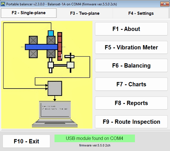
| Status-line text | Colour | What it means |
|---|---|---|
| “USB module found on” plus the port number | Green | The device is connected and responding |
| “USB module not connected” | Blinking yellow-orange | The device is not found and a background search is running |
| “USB module disconnected” | Orange | The cable was pulled out and the program is waiting for the device to return |
| “USB module on COM4 – not responding” | Orange | The COM port exists, but the firmware does not answer, usually because another program holds the port |
| “Firmware not supported on COM4” | Orange with red text | The device answers, but its firmware is below 5.5.0 and measurements are blocked |
Model, port and firmware are always on screen
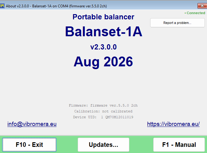
Next to the status line the program prints the device firmware as a line like firmware ver.5.5.0 2ch. The number is the version of the program inside the instrument, and 2ch or 4ch is the channel count, which is how the software knows whether to show Ch-3 and Ch-4 and how many correction planes to allow. The same three facts — model, COM port and firmware — are repeated in the title bar of every window, for example Balanset-1A on COM4 (firmware ver.5.5.0 2ch), so a screenshot taken during a job always carries its own provenance. The “F1 – About” window adds the device serial number, shown as Device UID.
Firmware 5.5.0 or newer is required
This version of the program measures only with device firmware 5.5.0 and newer. Older firmware is not supported, and that means both the old 4.10.x line and the intermediate 5.0.x to 5.4.x versions — an instrument that measured yesterday on firmware 5.2.0 is refused until it is updated. The refusal is explicit rather than silent. The device is still identified and its COM port is deliberately kept assigned to it, because the built-in updater needs that port. The status line turns orange with the red text “Firmware not supported on COMx”, the firmware version below it is shown in red, and once for each pair of port and firmware version the program asks “Update the device firmware now?”. Answer “Yes” and the “Updates” window opens. Until the firmware is updated, the mode buttons still work and the windows still open, but the live streams in the Vibration Meter and the Analyzer do not start and a balancing run is not accepted.
One consequence has to be stated plainly, because it affects data you may already own: archive records made on pre-5.x firmware can no longer be read correctly by this version. The files are intact, but the levels are displayed 16 times too small and on a different frequency scale, so such a record must not be treated as a measurement. Re-measure the machine on current firmware, or open the old record with an older version of the program.
Updating the firmware from the program
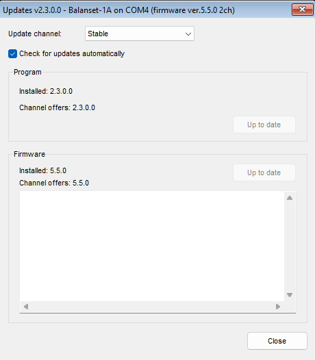
Firmware is updated from inside the application, with no third-party flashing utility: open “F1 – About”, press “Updates…”, and use the “Firmware” block. The program downloads the build for the selected channel, verifies its checksum and flashes the device; the whole operation takes 15 to 30 seconds, and the log field under the button shows the progress as “Downloading… NN%” followed by the flasher messages. Do not disconnect the device while it runs. When it finishes, “Firmware updated successfully.” appears and the link is restored automatically — there is no need to unplug the cable or restart the program, because the device is re-identified at once and the new version appears in the titles of all open windows. The channel count is re-read at the same time, since a firmware update can change it. If a previous attempt was interrupted and the device is stuck in the bootloader, the window recognises that state and reports “Bootloader detected (no firmware)”, and flashing it again is the standard recovery path.
Losing the cable is not a crash
Pulling the USB cable out mid-job is handled without blocking dialogs. The status line changes to “USB module disconnected”, a measurement in progress terminates cleanly and writes “ERROR: USB cable disconnected. Check USB connection.” into the session log, and a red “USB disconnected” caption appears in the measurement window. The background search keeps running, so plugging the cable back in restores the connection by itself, and a live stream that was running in the Vibration Meter or the Analyzer restarts automatically without reopening the window. Only an unfinished F9 capture has to be started again.
Program updates and support
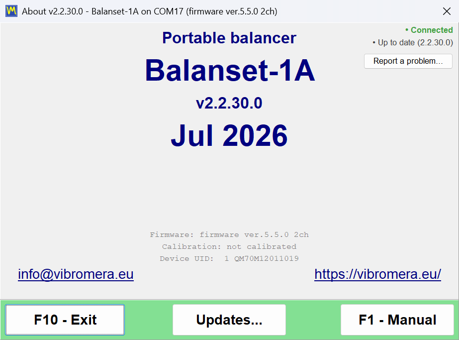
The program can keep itself current, and it tells you what it is doing. It checks for new versions on the updates.vibromera.com server over an HTTPS-only connection, in the background at startup and again when you open the “About” window, and the result is cached for 24 hours so the server is not called repeatedly. When a newer version exists on your channel, a “New version available” link appears in the bottom-right corner of the main window; when there is no update, that corner is simply empty. The automatic check can be switched off entirely with the “Check for updates automatically” checkbox in the “Updates” window, and with it off the program does not contact the server at all.
| Line in “About” | Meaning |
|---|---|
| “Connected” or “Offline” | Whether the update server is reachable; while the check runs it shows “Checking server…” |
| “Update available: X.Y.Z” | A new version exists; click the line to open the installation window |
| “Up to date” | The latest version is installed; clicking repeats the check at once, bypassing the 24-hour cache |
| “Update check failed” | The server is unreachable; the tooltip explains why and a click retries |
Installing an update
Clicking the link opens the “Update available” window, which shows the new version number, the “Current version”, the release date, the download size and the release notes. “Install now” starts the process and “Later” postpones it. The program downloads the package, verifies its integrity with a SHA-256 checksum, closes itself and hands the installation to the BsUpdater.exe helper, which reports its phase and a live file counter such as “Extracting… 1234 / 3288” while it works. The helper then replaces the files and launches the new version, which shows a short notification about the version that was installed. If a download fails, the window stays responsive and shows “Download failed:” with the reason, so you can fix the cause and retry.
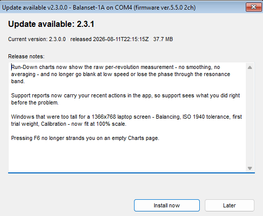
Your data is not touched by an update. The settings in Bs1A.cfg are preserved, the balancing archive is preserved because it lives in the user’s Documents folder, and report templates you have modified are saved alongside the new ones under names of the form name.user-*.htm, with the program listing them after the update. Note that those saved edits are not merged into the new template automatically, so a company letterhead has to be carried over by hand.
Rollback is built in as well. Before replacing anything, the helper stores a backup of the previous version in the bin\updates folder. An update interrupted by a power cut is either finished or cleaned up on the next launch, and as a last resort bin\BsUpdater.exe can be run manually to restore the previous version. You can also step back deliberately at any time with the “Roll back” button in the “Updates” window, which asks for confirmation before it acts. Windows asks for UAC confirmation only when the installation directory is not writable by the current user, such as Program Files; a portable installation or one under Documents updates without any prompt. And if you happen to start the program while the helper is running, the launch is refused with a window titled “Update in progress” — that is normal, and the next start does not treat it as an abnormal termination.
Update channels
| Channel | What it offers |
|---|---|
| “Stable” | Tested versions; the default and the recommended choice for production work |
| “Latest” | The most recent official release |
| “Experimental” | Preview builds, with an explicit warning that they may be unstable |
| “Legacy” | A pinned older program version for older hardware; the firmware block shows “No build on this channel” |
Reporting a problem from inside the program
Support is not an e-mail address you have to compose a description into from memory. Open “F1 – About”, press “Report a problem…”, and the “Send report to Vibromera support” window collects the technical context for you. You add a comment in the “Comment (optional):” field, attach screen captures with “Attach screenshots…” in PNG, JPG, BMP or GIF up to 25 MB in total, and decide about “Attach full log (bs1a.log + rotated)”. For an ordinary report that checkbox is on by default and worth leaving on, because the log is what shortens the diagnosis; for a complaint about a failed update it is effectively mandatory, since only that archive contains the update helper’s own log. A quick screenshot of any window is one key away: F12 writes a PNG into Documents\Bs1A\Screenshots.
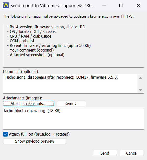
If the previous session ended abnormally, the next launch offers to send a report with a service comment already filled in, and for such a crash report the full-log checkbox is off by default so you can decide. An unfinished balancing job is not lost while this happens, because the session is auto-saved at every step and the program offers to restore it. If the server cannot be reached, the program offers to save the report as a support-report file with a timestamp in its name and opens Explorer at that file, so it can be sent by any other route. Pre-sales and compatibility questions can also go straight to a person over WhatsApp, at https://wa.me/37258364849.
Working offline, and what leaves your computer
The Balanset software is a local Windows program that talks to a USB device. There is no cloud service behind it, no account to create, no licence server to reach and no subscription to renew. Measuring vibration, running a balancing job, calculating correction weights, checking the result against ISO 1940 and producing the HTML protocol all happen on the laptop in front of you, and every one of them works with the network cable unplugged and Wi-Fi switched off. This matters in the places these instruments actually go: a ship’s engine room, a mine, a cement plant, a paper mill, a site where policy forbids connecting a foreign laptop to the plant network at all.
Only two things ever use the internet, and both are optional and both go to updates.vibromera.com over HTTPS only. The first is the update check, which can be switched off with “Check for updates automatically”, after which the program stops contacting the server. The second is a support report, which is only ever sent when you press “Send” yourself, and which requires an access token file installed with the program. Nothing is transmitted in the background beyond these two paths.
When you do send a support report, the contents are not a mystery. The window lists them, and the “Show payload preview” button shows the exact payload before anything is sent: the program version, the firmware version and the device UID; system information such as the operating system, language, DPI, displays, processor, memory and disk load and the list of COM ports; up to 50 KB of recent diagnostic log lines including your recent actions in the application; your comment; and the files you attached. The manual states the boundary explicitly, and so do we: session files and measurement results are not included in the report. Your customers’ machines, rotor names, vibration levels and balancing protocols stay on your disk unless you choose to attach them.
The same principle runs through the way the program stores things. Settings are a readable INI file rather than registry keys. The archive and the reports are ordinary files in Documents\BalSoft\Bs1A that you can back up, copy to another computer or hand to a client. Reports are UTF-8 HTML that opens in any browser on any operating system. Route Inspection files are plain files written in SI units with a decimal point regardless of the Windows regional format, so a route recorded on a German laptop reads correctly on a Turkish one. There is no proprietary container between you and your own measurements.
Get the instrument — the software is included
Both kits ship with this same program and its updates. No subscription, no per-seat licence, no cloud account. Two-year warranty, worldwide DHL shipping.
Balanset-1A — €1,975Balanset-4A, 4 channels — €6,803Ask an engineer (WhatsApp)
Frequently asked questions
Is the software sold separately, or is it included with the instrument?
The software is part of the kit and is not sold separately. Balanset-1A costs EUR 1,975 and Balanset-4A costs EUR 6,803, and both include the same Windows program plus updates from the vendor's update server. There is no subscription and no per-seat licence to renew.
Which instrument firmware does this version of the software require?
Firmware 5.5.0 or newer. On firmware 4.10.x and on the intermediate versions 5.0.x to 5.4.x the instrument is still detected and its COM port stays visible, but no measurement will start and balancing runs are rejected. The status line shows Firmware not supported on COMx, and the firmware can be updated from inside the program in 15 to 30 seconds.
Can the software balance in 3 or 4 correction planes?
Yes, but only under two conditions: the Balancing form on the F4 – Settings tab must be set to Modern, and the instrument must be the 4-channel Balanset-4A. The maximum number of correction planes equals the number of vibration channels, so the 2-channel Balanset-1A balances in 1 or 2 planes. The Classic form supports 1 and 2 planes in either case.
Does the software need an internet connection or a cloud account?
No. It is an ordinary local Windows program that reads the instrument through a USB COM port, and all measuring, calculating, archiving and reporting works fully offline with no registration. An internet connection is used only for two optional things: checking for program updates over HTTPS, and sending a support report if you choose to.
Which languages does the interface support?
The interface and the user manual are available in 27 languages, selected from the language list on the F4 – Settings tab. Changing the language requires a restart of the program. Unit symbols such as g, g*mm, mm/s and RPM, and standard designations such as ISO 1940, stay in their standard form in every language.
What is included in the kit besides the software?
The Balanset-1A or Balanset-4A USB module, one vibration transducer (accelerometer) per vibration channel, a laser optical tacho speed sensor, the USB cable and sensor cables, the user manual, and the Balanset program. The tacho sensor is powered through its cable from the instrument, so it needs no batteries.
When I balance the same rotor again, do I have to repeat the trial runs?
No. The influence coefficients are saved into the archive automatically, and loading them with F5 – Apply coefficients, or with Load Coefficients inside the balancing window, brings back the coefficients, trial masses, radii, fixed-position count and tolerance. Only Run 0 is then measured and the correction is calculated immediately. The saved coefficients are valid for the same machine and rotor type with unchanged sensor positions and running mode, so mark the trial weight location on the rotor during the first job.
What are the PC requirements, and do I need administrator rights?
Windows 7, 8, 10 or 11 in 32-bit or 64-bit, one free USB port, about 150 MB of free disk space, and a screen of at least 1024×768, with 1366×768 or higher recommended. Installation does not require administrator rights, and a portable copy can simply be unpacked, as long as it is not placed in Program Files. Settings are kept in a Bs1A.cfg file rather than in the Windows registry.
Are Route Inspection and Bump test ready for production use?
Both are marked experimental in the manual and are switched off by default; you enable them on the F4 – Settings tab. They are usable and documented, but should be treated as features in trial operation rather than mature modules. The Route Inspection forecast in particular is a straight-line extrapolation over the last few visits and is described in the manual as a rough estimate for maintenance planning, not a guaranteed time to failure.
In what formats can I export a report, and why does PDF export fail on some machines?
Reports export to PDF, HTML as a single file, HTML with an image folder, RTF and RVF, and the HTML files are UTF-8 so they open in any browser on any system. PDF export needs at least one Windows printer installed, because the printer driver is used only to compute the page layout; on a machine with no printer at all, enable Microsoft Print to PDF and the export will work.